Exercise files

Table of contents

• Parallel and Concurrent Programming with Java 1
  • 1 Parallel Computing Hardware
    • Sequential vs. parallel computing
    • Parallel computing architectures
      • Flynn’s taxonomy
      • SPMD and MPMD
    • Shared vs. distributed memory
      • Shared
        • UMA
        • NUMA
        • Summary of shared memory
      • Distributed
  • 2 Threads and processes
    • Thread vs. process
      • A process
      • Thread
      • Data sharing
      • Processes or Threads
    • Thread vs Process: Java Demo
    • Concurrent vs. parallel execution
      • Comparison
    • Execution scheduling
      • Scheduler
      • Context switch
      • Scheduling algorithms:
    • Execution scheduling: java demo
    • Thread lifecycle
    • THread lifecycle: Java demo
    • Thread attributes in Java
    • Runnable vs thread: java demo
      • The tradeoff
    • Daemon thread
    • Daemon thread: Java demo
  • 3 Mutual Exclusion
    • Data race
    • Data race: Java demo
    • Mutual exclusion
      • critical section
      • Mutex(lock)
      • Atomic operation
      • Acquiring a lock
    • Mutual exclusion: Java Demo
    • Atomic variable: Java demo
    • Synchronized method: Java demo
    • Synchronized statement: Java demo
      • The right way
      • The wrong way
      • A trap
    • Summary
  • 4 Locks
    • Reentrant lock
    • Reentrant lock: Java demo
      • Demo lock and unlock on time
      • Demo lock/unlock more than once
    • Try lock
    • Try lock: Java demo
    • Read-write lock
      • An example
      • When to use a read-write lock
    • Read-write lock: Java demo
  • 5. Liveness
    • Deadlock
    • Deadlock: Java demo
    • Abandoned lock
    • Abandoned lock: Java demo
    • Starvation
    • Starvation: Java demo
    • Livelock
    • Livelock: Java demo
• Parallel and Concurrent Programming with Java 2
  • Intro
  • 1.Synchronization
    • Condition variable
      • Conceptually
      • implementing a shared queue or buffer
    • Condition variable: Java demo
      • Using a conditiona variable
      • Signaling a Condition Variable
    • Producer–consumer
      • Rate of consumer vs producer
      • Simple producer-consumer setup can expand into a pipeline of tasks.
    • Producer–consumer: Java demo
    • Semaphore
      • Operation acquire()
      • Operation release()
      • Example
      • Counting semaphore
      • Binary Semaphore
    • Semaphore: Java demo
  • 2. Barriers
    • Race condition
      • Data race vs race condition
      • Example
      • Race condition is a Heisenbug
    • Race condition: Java demo
    • Barrier
    • Barrier: Java demo
      • CyclicBarrier
      • Transcript
    • CountDownLatch: Java demo
      • CyclicBarrier vs CountDownLatch
      • Java demo
      • Common useage of CountDownLatch
  • 3. Asynchronous Tasks
    • Computational graph
      • Spawn/fork
      • Sync/join
    • Thread pool
      • Intro
      • Use a thread pool
    • Thread pool: Java demo
      • Exercise
      • Transcript
    • Future
      • Transcript
    • Future: Java demo
      • Transcript
    • Divide and conquer
      • Transcript
    • Divide and conquer: Java demo
• TODO: 03_07 code - Transcript
  • 4. Evaluating Parallel Performance
    • Speedup, latency, and throughput
      • Reasons for parallelism
      • 3 metrics
      • Caveat
    • Amdahl’s law
      • parallel isn’t always best, benefitial or even necessary
    • Measure speedup
      • Recomendation for benchmarking
      • Transcript
    • Measure speedup: Java demo
      • Transcript
        • code for Measure sequential
        • code for measure Parallel
      • code for display and compare results
      • run program
      • compare and improve
  • 5.Designing Parallel Programs
    • Partitioning
      • Transcript
    • Communication
      • high-level structures
      • A few factors to consider
      • Transcript
    • Agglomeration
      • Granularity
      • keep flexibility in mind
      • Transcript
    • Mapping
      • Use case
      • Goal and strategies
      • Transcript
    • Summary
  • TODO: review everything!!!
  • 6. Challenge Problems
    • Welcome to the challenges (Transcript)
    • Challenge: Matrix multiply in Java (Transcript)
• TODO

Parallel and Concurrent Programming with Java 1

Intro

1 Parallel Computing Hardware

Sequential vs. parallel computing

Sequential

• simple, straight forward
• not taking advantage of the parallel hardware

Parrallel

• Higher throughput:
  • same task faster
  • or more tasks in same time
• need extra effort for coordination

Parallel computing architectures

One of the most widely used systems for classifying multiprocessor architectures is Flynn’s taxonomy

Flynn’s taxonomy

Flynn’s taxonomy distinguishes four classes of computer architecture based on two factors

• the number of concurrent instruction or control streams

• the number of data streams

• SIMD stands for Single Instruction, Multiple Data.
• Single Instruction, Single Data or SISD architecture: a sequential computer with a single processor unit. The simplest of these four classes
• Single Instruction, Multiple Data, or SIMD, which is a type of parallel computer with multiple processing units. All of its processors execute the same instruction at any given time, but they can each operate on different data element.
  • SIMD architecture is well-suited for applications that perform the same handful of operations on a massive set of data elements like image processing. And most modern computers use graphic processing units or GPUs with SIMD instructions to do just that.
  • e.g. As an SIMD computer, our two processors are both executing the same chopping instruction, but I’m chopping celery as my data while Baron chops a carrot. - And we’ll execute those instructions in sync with each other. (chopping)
• Multiple Instruction, Single Data or MISD(not very useful), each processing unit independently executes its own separate series of instructions. However, all of those processors are operating on the same single stream of data. MISD doesn’t make much practical sense, so it’s not a commonly used architecture.
• Multiple Instruction, Multiple Data or MIMD computer, every processing unit can be executing a different series of instructions, and at the same time, each of those processors can be operating on a different set of data. MIMD is the most commonly used architecture in Flynn’s taxonomy, and you’ll find it in everything from multicore PCs to network clusters and supercomputers. Now, that broad MIMD category is sometimes further subdivided into two parallel programming models, which also have four letter names.
  • Single Program, Multiple Data, or SPMD
  • Multiple Program, Multiple Data, MPMD.

SPMD and MPMD

Instead of differentiating at instruction level, SPMD and MPMD differ at the program level

In the SPMD model, multiple processing units are executing a copy of the same single program simultaneously. However, they can each use different data. That might sound a lot like the SIMD architecture from earlier, but it’s different because although each processor is executing the same program, they do not have to be executing the same instruction at the same time. The processors can run asynchronously and the program usually includes conditional logic that allows different tasks within the program to only execute specific parts of the overall program.

If Olivia and I are both following the same recipe or program, I can execute part of it, while Olivia’s processor handles a different task.

This SPMD model is the most common style of parallel programming and when we show you programming examples later in this course, we’ll structure the code as a single program and execute it on a multicore desktop computer, which is an MIMD architecture.

Multiple Data or MPMD model. In this scenario, processors can be executing different, independent programs at the same time while of course also be operating on different data.

Typically in this model, a divide and conquer approach is applied.

• one processing node will be selected as the host or manager, which runs one program that farms out data to the other nodes running a second program.
• Those other nodes do their work and return their results to the manager.

MPMD is not as common as SPMD, but it can be useful for some applications that lend themselves to functional decomposition, which we’ll cover later on.

Shared vs. distributed memory

In addition to a parallel computer’s architecture which can be categorized using Flynn’s taxonomy, another aspect is Memory. It’s important to understand

• how the memory is organized
• how the computer accesses data

Constraints when working with memory

• Speed: memory usually much slower than processors
• Mutex: when one processor is reading or writing to memory, that often prevents any other processors from accessing that same memory element

There are two main memory architectures that exist for parallel computing, shared memory and distributed memory.

Shared

In a shared memory system, all processors have access to the same memory as part of a global address space. Although each processor operates independently, if one processor changes a memory location, all of the other processors will see that change.

the term shared memory doesn’t necessarily mean all of this data exists on the same physical device. It could be spread across a cluster of systems. The key is that both of our processors see everything that happens in the shared memory space.

Based on how the processors are connected to memory and how quickly they can access it, shared memory is often classified into one of two categories

• uniform memory access
• nonuniform memory access

UMA

In a uniform memory access or UMA system, all of the processors have equal access to the memory, meaning they can access it equally fast.

There are several types of UMA architectures, but the most common is a symmetric multiprocessing system or SMP. An SMP system has two or more identical processors which are connected to a single shared memory often through a system bus. In the case of modern multicore processors, which you find in everything from desktop computers to cell phones, each of the processing cores are treated as a separate processor. For this course, we’ll be focused on parallel programming within the SMP architecture. And the example code we show you will be running on a multicore desktop computer.

Now, in most modern processors, each core has its own cache, which is a small, very fast piece of memory that only it can see, and it uses it to store data that it’s frequently working with. However, caches introduce the challenge that if one processor copies a value from the shared main memory, and then makes a change to it in its local cache, then that change needs to be updated back in the shared memory before another processor reads the old value, which is no longer current. This issue, called cache coherency, is handled by the hardware in multicore processors, so we will not go into detail on it for this course, but it’s something you should be aware of if you find yourself working with larger, more complex parallel computing systems.

NUMA

The other type of shared memory is a nonuniform memory access or NUMA system, which is often made by physically connecting multiple SMP systems together. The access is nonuniform because some processors will have quicker access to certain parts of memory than others. It takes longer to access things over the bus. But overall, every processor can still see everything in memory.

Summary of shared memory

• advantage: easier for programming in regards to memory, because it’s easier to share data between different parts of a parallel program.
• The downside is that they don’t always scale well. Adding more processors to a shared memory system will increase traffic on the shared memory bus, and if you factor in maintaining cache coherency, it becomes a lot of communication that needs to happen between all the parts.
• In addition to that, shared memory puts responsibility on the programmer to synchronize memory accesses to ensure correct behavior, but we’ll look into that later.

Distributed

In a distributed memory system, each processor has its own local memory with its own address space, so the concept of a global address space doesn’t exist. All the processors are connected through some sort of network, which can be as simple as Ethernet. Each processor operates independently, and if it makes changes to its local memory, that change is not automatically reflected in the memory of other processors.

• Disadvantage: change not automatically reflected on other nodes, and the programmer to explicitly define how and when data is communicated between the nodes
• advantage: it’s scalable. When you add more processors to the system, you get more memory too.

This structure makes it cost-effective to use commodity, off-the-shelf computers, and networking equipment to build large distributed memory systems. Most supercomputers use some form of distributed memory architecture or a hybrid of distributed and shared memory.

But for this course, we’ll stick with simple shared memory in an SMP architecture.

TO review

2 Threads and processes

Thread vs. process

When a computer runs an application, that instance of the program executing is referred to as a process.

A process

• includes: code, data, and state information.
• independent instance of a running program
• separate address space in memory.

An operating system’s job is to manage hundreds of active processes at once. -

Thread

Now, within every process, there are one or more smaller sub elements called threads.

• independent path of execution; a different sequence of instructions
• it can only exist as part of a process
• OS schedule threads for execution: threads are the basic units that the operating system manages and it allocates time on the processor to actually execute them.

Data sharing

Threads that belong to the same process share the processes’ address space, which gives them access to the same resources in memory including the program’s executable code and data.

You can think of the kitchen that our two threads are working in like the shared address space for our process. We both have direct access to the same cookbooks containing our instructions or code, and the ingredients that we’re cooking with represents the data and variables we’re manipulating. The ability for both of us to use these resources is certainly convenient, and it enables us to easily work together, but it does create the potential to cause problems if we don’t coordinate our actions, as we’ll see later in this course.

Sharing resources between separate processes is not as easy as sharing between threads in the same process, because every process exists in its own address space

its own separate kitchen. In this process, our two threads are making a salad, but that other process next-door is running a different program. Those threads are baking a cake. - Our variables and data are isolated to this address space, this kitchen, so the threads in the other process can’t directly access our salad data.

There are ways to communicate and share data between processes, but it requires a bit more work than communicating between threads. You have to use system-provided inter-process communication(IPC) mechanisms like

• sockets and pipes
• allocating special inter-process shared memory space
• remote procedure calls which is beyond the scope of what we’ll be discussing in this course.

Processes or Threads

Which is better - it depends

a rule of thumb, if you can structure your program to take advantage of multiple threads, stick with using threads rather than multiple processes.

• Threads are “lightweight” - requires less overhead to create and terminate than a process
• usually faster for an operating system to switch between executing threads from the same process than to switch between different processes.

Thread vs Process: Java Demo

Exercise: 02_02

JVM

• each java application executes within its own instance of JVM
• Each JVM instance is a separate, independent process

JVM creates additional threads to handle stuff, gabage collection etc.

Concurrent vs. parallel execution

Just because a program is structured to have multiple threads or processes does not mean they’ll necessarily execute in parallel.

Concurrency refers to the ability of a program to be broken into different parts that can run independently of each other, executed out of order or partially out of order without affecting the end result.

Concurrency is about how a program is structured and the composition of independently executing processes.

Consider this recipe to make a salad, which includes several steps that involve slicing and chopping vegetables. We can decompose those steps into a collection of concurrent tasks because the relative order in which we do them doesn’t matter. They’re order independent. To keep things simple, let’s just focus on two of those tasks for now. I’ll chop onions. - And I’ll slice cucumbers. This knife represents our computer’s processor. We only have one knife, so this is a single core processor. And only one of us will be able to execute our vegetable chopping routine at any given time. - We’ll have to take turns. You go first. - Thanks. My thread will use a processor to execute and slice some cucumbers. Then, after a bit, we’ll swap places. - Now my thread gets some time to execute and slice onions. - I want to slice now. - So we’ll swap places again, and we’ll keep on doing this until we’re both done.

In this scenario, we’re running concurrently because our two independent processes overlap in time. However, since we only have a single processor, only one of us will actually be executing at any instant in time. If we swap places and take turns more frequently, it might create the illusion that we’re executing simultaneously on our single processor, but this is not true parallel execution.

To actually execute in parallel, we need parallel hardware. In our kitchen, that means another knife and cutting board, a second processor.

In regards to computers, parallel hardware can come in a variety of forms.

• Most modern processors have multiple processing cores
• GPUs, contain hundreds, or even thousands, of specialized cores working in parallel to make amazing graphics that you see on the screen
• computer clusters distribute their processing across multiple systems.

Since we’ve structured ourselves as concurrent operations, I can begin slicing cucumbers with this processor. - While I cut onions with the other one. Now we’re actually executing in parallel because we’re both executing at the same time. And, as a result, we’re able to finish the job faster.

Comparison

Concurrency:

• program structure
• being able to deal with multiple things at once(illusion at least)

Parallelism

• simultaneous execution
• actually doing multiple things at once. Those things could be related, like chopping vegetables, but they don’t have to be.

Concurrency enables a program to execute in parallel, given the necessary hardware. But a concurrent program is not inherently parallel.

And programs may not always benefit from parallel execution

For example, the software drivers that handle I/O devices, like a mouse, keyboard, and hard drive, need to execute concurrently. They’re managed by the operating system as independent things that get executed, as needed. In a multi-core system, the execution of those drivers might get split amongst the available processors. However, since I/O operations occur rather infrequently, relative to the speed at which computer operates, we don’t really gain anything from parallel execution. Those sparse independent tasks can run just fine on a single processor, and we wouldn’t feel a difference.

Concurrent programming is useful for I/O-dependent tasks

like graphical user interfaces. When the user clicks a button to execute an operation, that might take a while. To avoid locking up the user interface until it’s completed, we can run the operation in a separate concurrent thread. This leaves the thread that’s running the UI free to accept new inputs.

That sort of I/O-dependent task is a good use case for concurrency. Parallel processing really becomes useful for computationally intensive tasks, such as Matrix multiplication.

Execution scheduling

Scheduler

The OS includes a scheduler that controls when different threads and processes get their turn to execute on the CPU. The scheduler makes it possible for multiple programs to run concurrently on a single processor.

When a process is created and ready to run, it gets loaded into memory and placed in the ready queue. Think of these as cooks in the kitchen that are ready to work.

The scheduler is like the head chef that tells the other cooks when they get to use the cutting board.It cycles through the ready processes so they get a chance to execute on the processor. If there are multiple processors, then the OS will schedule processes to run on each of them, to make the most use of the additional resources.

• A process will run until it finishes, and then the scheduler will assign another process to execute on that processor.
• Or, a process might get blocked and have to wait for an I/O event, in which case it will go into a separate I/O waiting queue, so another process can run.
• Or, the scheduler might determine that a process has spent its fair share of time on the processor, and swap it out for another process from the ready queue. When that occurs, it’s called a context switch.

Context switch

The operating system has to

• save the state, or context, of the process that was running, so it can be resumed later,
• load the context of the new process that’s about to run.

If I’m a process that’s executing on this processor to chop cucumbers, when a scheduler decides it’s time for a context switch, I’ll need to pause what I’m doing and store the state of that task. - And as the new process that just got scheduled, I’ll load my state information and then begin executing.

context switches are not instantaneous. It takes time to save and restore the registers and memory state, so the scheduler needs a strategy for how frequently it switches between processes.

Scheduling algorithms:

• First come, first served
• shortest job next
• priority
• shortest remaining time
• round-robin
• multiple-level queues

Some of these algorithms are preemptive, which means they may pause, or preempt, a running, low-priority task when a higher priority task enters the ready state. In non-preemptive algorithms, once a process enters the ready state, it’ll be allowed to run for its allotted time.

Which algorithm a scheduler chooses to implement will depend on its goals. Some schedulers might try to maximize throughput, or the amount of work they complete in a given time

others might aim to minimize latency, to improve the system’s responsiveness.

Different operating systems have different purposes, and a desktop OS like Windows will have a different set of goals and use a different type of scheduler than a real-time OS for embedded systems.

While it’s important to understand the concept of scheduling, and that it’s taking place, you usually don’t need to worry about the nitty-gritty details of how the scheduler works, because it’s often handled under the hood by the operating system. In fact, you might not have any control over when the parts of your program actually execute. - And that’s an important thing to keep in mind. Avoid running programs expecting that multiple threads or processes will execute in a certain order, or for an equal amount of time, because the operating system may choose to schedule them differently from run to run.

Execution scheduling: java demo

02_05

To demo: You can see that each time we run this, we’re getting a different result. So scheduling is not always consistent, so you shouldn’t rely on it for threads to be executed in equal amount of time or in a particular order.

Thread lifecycle

When a new process or program begins running, it will start with just one thread, which is called the main thread, because it’s the main one that runs when the program begins. That main thread can then start or spawn additional threads to help out, referred to as its child threads, which are part of the same process but execute independently to do other tasks. Those threads can spawn their own children if needed, and as each of those threads finish executing, they’ll notify their parent and terminate, with the main thread usually being the last to finish execution. fou

four states of thread life cycle

• new: not actually running and doesn’t take CPU resources
• runnable
  • Some programming languages require you to explicitly start a thread after creating it
  • once the thread is started, it’s in runnable state: meaning the operating system can schedule it to execute
  • Through contact switches, runnable threads get swapped out with other threads to run on one of the available processors
• blocked
  • When a thread needs to wait for an event to occur, like an external input or a timer, it goes into a blocked state while it waits.
  • Blocked does not using any CPU resources
  • The operating system will return it to the runnable state when condition meets
  • Parent call join() method to wait for child threads to finish. join() sends the parent into blocked state, until child thread notifies it.
• terminated: A thread enters the terminated state when it either completes its execution or is abnormally aborted

If I’m the main thread in this kitchen, and I spawn or create another thread to help me, that child thread will begin in the new state. - Hello! - This thread isn’t actually running yet, so it doesn’t take any CPU resources. - I don’t even know what I’m supposed to be doing. Part of creating a new thread is assigning it a function, the code it’s going to execute. Olivia, I need you to slice these sausages, we’re making soup. - I can do that. I’m ready to start. - Right, you can start now. Some programming languages require you to explicitly start a thread after creating it. - [Olivia] Now that I’ve started, I’m in the runnable state, which means the operating system can schedule me to execute. Through contact switches, I’ll get swapped out with other threads to run on one of the available processors. - Olivia is running independently now, so my thread is free to continue executing my own tasks, when it’s my turn to get scheduled on the processor. (sausage taps) - Oh man, this sausage is frozen. I need to wait for it to thaw before I can continue. When a thread needs to wait for an event to occur, like an external input or a timer, it goes into a blocked state while it waits. The good thing is that, while I’m blocked, I’m not using any CPU resources. The operating system will return me to the runnable state when the sausage is thawed. - And that frees up the processor for other threads to use. Now my thread may eventually reach a point where I need to wait until one of my children threads has finished for me to continue on. Maybe I’ve finished preparing everything else. I’ve completed all of my tasks, and I need Olivia to finish slicing the sausage. I can wait for her thread to complete its execution by calling the join method. When I call join, my thread will enter a block state, waiting until Olivia’s done. Ah, the sausage is finally thawed. Now I’ll go back to the runnable state and continue executing. (tape whirs) Now I’ve finished executing, so I’ll notify my parent thread that I’m done. Hey Barron, I’m done! And then I’ll enter the final terminated state. (sighs) A thread enters the terminated state when it either completes its execution or is abnormally aborted. - Since Olivia notified me that she’s done, I’ll return to the runnable state, so I can continue preparing soup.

Different programming languages may use different names for their states, and have a few additional ones, but in general, new, runnable, blocked, and terminated are the four phases of the life cycle of a thread.

THread lifecycle: Java demo

Six states of java thread

• NEW
• RUNNABLE
• BLOCKED
• WAITING(special blocked state)
• TIMED_WAITING(special blocked state)
• TERMINATED

Exercise file: 02_07

/**
 * Two threads cooking soup
 */

class ChefOlivia extends Thread {
    public void run() {
        System.out.println("Olivia started & waiting for sausage to thaw...");
        try {
            Thread.sleep(3000);
        } catch (InterruptedException e) {
            e.printStackTrace();
        }
        System.out.println("Olivia is done cutting sausage.");
    }
}

public class ThreadLifecycleDemo {
    public static void main(String args[]) throws InterruptedException {
        System.out.println("Barron started & requesting Olivia's help.");
        Thread olivia = new ChefOlivia();

        System.out.println("Barron tells Olivia to start.");
        olivia.start();

        System.out.println("Barron continues cooking soup.");
        Thread.sleep(500);

        System.out.println("Barron patiently waits for Olivia to finish and join...");
        olivia.join();

        System.out.println("Barron and Olivia are both done!");
    }
}

Key points

• methods on a thread
  • .start()
  • .join()
  • .getState()
• methods on Thread
  • Thread.sleep(s)

Thread attributes in Java

• threads state: retrieved using the Thread.state getState()
• Thread currentThread(), returns a reference to the currently executing thread object. You then can access that thread
• Thread ID: Whenever a new thread gets created, it will be assigned a thread ID.
  • positive, long number
  • a unique identifier for the thread, and remains unchanged during it’s lifetime.
  • long getID()
  • after a thread terminates, that ID number will be available for other new threads to reuse
• Threads name: a string that can be used for identification purposes.
  • Multiple thread can have the same name, but they’ll never have the thread ID.
  • Several thread constructor method that allow you to specify the name when creating a thread
  • If a name is not specified, java will generate a new name for the thread, usually with a default format like Thread-N, where N is a positive integer.
  • setName() to change a threads name after creating it
  • getName() retrieve name
• Priority: which tells the java virtual machines thread scheduler when each thread should run relative to other threads
  • range from 1 to 10, 1 lowest, 10 highest.
  • setPriority() and getPriority() methods respectively
• Java threads do not maintain a reference to their parent thread.
  • When a new thread is created, it’s parent is used to set properties like the threads priority and it’s demon status, which we’ll cover later. But the child does not maintain a reference to it’s parent thread.
  • One reason for that is that it enables the parent thread to be garbage collected by the jvm to reclaim memory, which would not be possible if the child thread was holding a reference to it.

Runnable vs thread: java demo

Creating threads in Java

• Extend the Thread class
• Implement the Runnable interface

Runnable interface

• interface for a class that will be executed by a thread. Thread itself implements Runnable
• requires a void run() method

02_09

The tradeoff

• Extending thread
  • cannot extend additional classes, because java doesn’t allow multiple inheritance
  • each instance is a separate object
• Implementing Runnable
  • can implement other interfaces and extend a class
  • multiple threads can share a single Runnable object
    • benefit of reduce memory usage
    • be mindful any instance variable in the runnable object, will be shared, used and affected by all threads.

In general, using Runnable is better, and align with the design principle of coding to a interface instead of an implementation.

Using Thread may end up with simpler code, and can be used where using Runnable doesn’t benefit much.

Daemon thread

We often create threads to provide some sort of service, or perform a periodic task in support of the main program. A common example of that is garbage collection.

A garbage collector

• is a form of automatic memory management
• runs in the background
• attempts to reclaim garbage, or memory that’s no longer being used by the program

Why you don’t want to spawn your own normal thread for garbage collection?

• thread for garbage collection runs in a continuous loop, and never exit
• spawning it as a normal child thread, means main thread will be stuck waiting for this child thread

Many languages include garbage collection as a standard part of their run time environment, but for this demonstration, I’ll spawn my own new thread to handle garbage collection. - Man, what a mess. - Olivia is a separate child thread that will execute independently of my main thread. So, I can continue doing what I’m doing here, getting my soup ingredients ready. - While I try to reclaim some memory, or counter space, by clearing out Baron’s garbage. - This set-up, with Olivia running as a separate thread to provide that garbage collection service, will work fine until I’m ready to finish executing. Bam, now my soup’s spiced and ready, my main thread is done executing, and I’m ready to exit the program. But I can’t. - Because I’m still running. Since Baron spawned me as a normal child thread, he won’t be able to exit until I’ve terminated. - And since Olivia’s thread is designed to collect garbage in a continuous loop, she’ll never exit. I’ll be stuck here waiting forever, and this process will never terminate.

Threads that are performing background tasks, like garbage collection, can be detached from the main program by making them what’s called a daemon thread.

Daemon(Background) thread

• is a thread that will not prevent the program from terminating.
• By default, new threads are usually spawned as non-daemon or normal threads, and you have to explicitly turn a thread into a daemon or background thread.

Olivia, I forgot to tell you this earlier, but you’re a daemon thread. - Oh man, you detached me. - When my main thread is finished executing and there aren’t any non-daemon threads left running, this process can terminate. And Olivia’s daemon thread will terminate with it. - Since I was terminated abruptly with the process, I didn’t have a chance to gracefully shut down and stop what I was doing. That’s fine in the case of a garbage collection routine, because all of the memory this process was using will get cleared as part of terminating it. But if I was doing some sort of IO operation, like writing to a file, then terminating in the middle of that operation could end up corrupting data.

If you detach a thread to make it a background task, make sure it won’t have any negative side-effects if it prematurely exits.

Daemon thread: Java demo

02_11

• use .setDaemon(true) to change a thread’s daemon status before starting it
• new threads will inherit daemon status from their parent
• Daemon threads doesn’t terminate gracefully. When JVM halts, any remaining daemon threads are abandoned. Use daemon threads sparingly
  • example, don’t use daemon threads for IO, because if daemon thread exits unfinished write/update may cause corrupted data.

3 Mutual Exclusion

Data race

One of the main challenges of writing concurrent programs is identifying the possible dependencies between threads to make sure they don’t interfere with each other and cause problems.

Data race

1. when two or more threads are concurrently accessing the same location in memory
2. and at least one of those threads is modifying it.

How to recognize the data race.

Read-modify-write is a common scenario

• thread 1 read, modify gets paused, - - - - - - - - - - - - - write.
• thread 2 - - - - - - - - - - - - - -, read, modify, write.

Olivia and I are two concurrent threads working together to figure out what we need to buy from the grocery store. I’ll take inventory of the pantry and when I see that we’re running low on something, I’ll add more of that item to our shared shopping list. - While Barren does that, I’ll look through my recipe book and I’ll add ingredients to our shopping list for the meals that I wanted us to cook this week. - Even though we’re two separate threads doing different tasks, we run the risk of a data race because we’re both accessing and modifying the same shared recourse. (paper flutters) Our shopping list. Now, to the panty! - Oh! This garlic mashed potato recipe looks delicious, I’ll need five potatoes for it. I see that our shopping list already has three potatoes on it. Three plus five is eight. So, I’ll erase three (pencil scribbles) and write down eight. As you can see, even a simple operation, like adding two numbers is actually a multiple step process. First, I had to read the existing value of the item from the shopping list. Then, I modified the value by adding what I needed to it. Finally, I wrote the result back to the shopping list. - It looks like we’re running low on garlic in the pantry. I think we should restock it with two more cloves. I see that there is currently one clove of garlic on the list. One plus two is uh… - My garlic mashed potato recipe calls for five cloves of garlic. I see there’s currently one clove of garlic on the list, one plus five is six. So, I’ll update the list to have six cloves on it. (pencil scribbles) - Three! One plus two is three. We need three cloves of garlic. (pencil scribbles) - Now, we have a problem. The shopping list started with one clove of garlic. Barren wanted to add two more and I needed to add five more. One plus two plus five means we should’ve ended up with eight cloves of garlic on this list. But somehow, we only have three. I need more garlic for my mashed potatoes. - We just had a data race. As concurrent threads, it’s up to the operating system to schedule when we each get to execute. Right after I read the value of one from that shared shopping list, my thread got paused. - Then my thread became active and changed the number of garlic from one to six. - And finally, my thread became active again and at that point, I was operating with old data in my local memory because I thought the existing value of garlic on the shopping list was still one. So, I finished my operation by changing it to three.

In this example, it was the unfortunate timing of when our threads were scheduled that caused the problem. But, the unpredictability of when threads get scheduled means sometimes the data race will occur and cause problems but other times, everything might work just fine. That inconsistency makes data races a real challenge to recognize and debug.

Data race: Java demo

03_02

Even though the simple garlicCount++ operation is only a single line of code, in the background, the computer is actually performing a three-step read, modify, write process. My two concurrent threads end up stepping on each other and unintentionally overwriting each other’s changes to produce an incorrect result.

• Detecting data races is hard, there are tools out there, and certain languages may have additional feature for detecting it
• Preventing data races in the first place. Since a data race only occurs when at least one of the concurrent threads is modifying the value of a memory location, pay close attention to anywhere you use an assignment operation or an operator like the ++ which increments and changes the variable’s value. If there is a potential that two or more threads could access that variable, then you will almost certainly need to use some form of synchronization.

Mutual exclusion

Anytime multiple threads are concurrently reading and writing a shared resource, it creates the potential for incorrect behavior, like a data race. But we can defend against that by identifying and protecting critical sections of code.

critical section

• A critical section or critical region is part of a program that accesses a shared resource, such as a data structure memory, or an external device, and it may not operate correctly, if multiple threads concurrently access it.
• The critical section needs to be protected so that it only allows one thread or process to execute in it at a time.

Barron and I experienced a data race as we added garlic to our shared shopping list, because incrementing a value is actually a three-step process. Read the current value, modify it, and then write back the result. Those three steps are critical section, and they need to execute as an uninterrupted action, so we don’t accidentally override each other.- I have an idea. Give me your pencil. - Hey, I was using that. - Now there’s only one pencil for us to share, and the rule is that only the person holding the pencil can access the shopping list, either to read or write it. That way, one of us won’t accidentally read a wrong value, because the other one is only halfway done updating it. In this arrangement, the pencil is serving as a mechanism called a mutex, short for mutual exclusion, which you’ll also hear referred to as a lock.

Mutex(lock)

• Mechanism to implement mutual exclusion
• Only one thread or process can have possession of the lock at a time
• Thus limiting access to critical section, preventing multiple threads from simultaneously accessing a shared resource, forcing them to take turns.

If either of us wants to access the shopping list, we first need to pick up the pencil, to acquire the lock on it. We do whatever we need to with the shared notepad, and then when we’re done, release the lock by putting down the pencil.

Atomic operation

• Execute as a single action, relative to other threads
• cannot be interrupted by other concurrent threads

The operation to acquire the lock is an atomic operation, which means it’s always executed as a single, indivisible action. To the rest of the system, an atomic operation appears to happen instantaneously, even if under the hood, it really takes multiple steps. The key here is that the atomic operation is an uninterruptible.

So, if I grab the pencil. - Acquiring the mutex is an atomic action that no other thread can interfere with halfway through. Either you have the mutex, or you don’t. And now that you do have a lock on our pencil, you can safely execute in the critical section. - I see we already have 10 carrots on the list. I’ll add five more to that. - Oh, and we’re going to need some more onions too. - Well, I currently possess a mutex, so you’ll have to wait until I’m done.

Acquiring a lock

Threads that try to acquire a lock that’s currently possessed by another thread, can block/wait till it’s available.

There, I’m done with the notepad for now. So, I’ll release the lock. - And I’ll acquire the lock, so I can add onions to the list. - Don’t forget to release the mutex when you’re done. - Okay.

Keep protected sections of code as short as possible.

Since threads can get blocked and stuck waiting for a thread in the critical section to finish executing, it’s important to keep the section of code protected with the mutex as short as possible. If I take the pencil, execute a critical section by adding more lettuce, and then hold on to the pencil while I contemplate what else to buy. - I’m stuck waiting for Olivia to return the pencil so I can use it, and getting kind of annoyed. - Only thinking about what I want to buy doesn’t actually require the shared notepad. So the operation doesn’t require mutual exclusion. I should have returned the pencil as soon as I was done updating the list. That way Barron could use it to execute the critical section, while I’m busy doing other things.

Mutual exclusion: Java Demo

03_04

• add import java.util.concurrent.locks.*;
• static Lock pencil = new ReentrantLock();: more on ReentrantLock in next 4. Locks
• add pencil.lock() and pencil.unlock() to the thread’s run() method, before and after the critical section

Atomic variable: Java demo

03_05

Java Atomic package Their values update as a single, uninterrupted operation which makes them “thread-safe.”

• simpler than using a lock to protect shared var
• classes that support lock-free, thread safe programming on single variables
• a lot of available types, each has a variety of methods that implement Atomic versions of most standard operations.
  • AtomicBoolean
  • AtomicInteger
  • AtomicIntegerArray …
• import java.util.concurrent.atomic.*
• static AtomicInteger garlicCount = new AtomicInteger(0);
• garlicCount.incrementAndGet()

Synchronized method: Java demo

Intrinsic Locks

Transcript: Something unique in Java is that every object has an intrinsic lock associated with it, a thread that needs exclusive access to an object’s fields has to acquire that object’s lock before accessing them and then release that intrinsic lock when it’s done.

The Java programming language provides two basic synchronization constructs to use those intrinsic locks

• synchronized methods
  • add the keyword synchronized to the method’s declaration
  • Multiple invocation will not interleave. Avoid multiple threads invoking the same method and interleaving the execution.
  • When a thread tries to invoke a synchronized method while another thread is executing a synchronized method for that same object, the second thread will suspend execution until the first thread is done and exits.
• synchronized statements(next chapter)

03_06

To demonstrate that in Java, I’ll modify the previous example program to show a data race in which two concurrent threads increment a shared counter variable 10 million times each. Within the shopper class, I’ll create a new static method called addGarlic and I’ll include the synchronized keyword in its declaration. Next, I’ll put the operation to increment the garlicCount variable inside of that synchronized method. And finally, I’ll replace the call to garlicCount++ in the for loop on line 15 with a call to the synchronized addGarlic method. I’ll run the program. And good news! I get the correct output of 20 million. Only one of the two concurrent threads can execute within the synchronized addGarlic method at a time so the program avoids a data race.

Now an important thing to note in this example is that I marked the addGarlic method as static so that it’s associated with the shopper class and not a specific instance of a shopper. By doing so, when either thread invokes the synchronized addGarlic method, it will acquire the intrinsic lock that’s associated with the class object. If I remove the static keyword on line nine, then each of the two shopper threads will invoke their own instance of the addGarlic method which is associated with their own object’s intrinsic lock. If I run the program now, it does not work correctly. The threads are no longer using the same intrinsic lock so I end up with a data race.

Synchronized statement: Java demo

When creating an synchronized statement, you specify the object that will provide the intrinsic lock.

synchronized (object) {
    //protected code
}

Before a thread can execute the code contained within the synchronized statement, it must first acquire the intrinsic lock associated with the specified object and then when the thread is done, it will release its hold on that lock.

03_07

The right way

I want to synchronize access to line 11 which increments the shared garlicCount variable. So I’ll wrap that line in a synchronized statement and I’ll give it the shopper.class object to use for the intrinsic lock. When I run this program both threads will be acquiring and releasing the same intrinsic locks associated with the shopper class before and after they increment the garlicCount. So I get the expected output value of 20 million.

The wrong way

Now let’s see what happens if instead of using the shopper class object, I use each instance of the shopper as the object for the synchronized statement. To do that, we’ll replace shopper.class with the this keyword. Now when I run the program, I get an incorrect result because each of the two shopper threads is acquiring and releasing the intrinsic lock associated with their own instances. They’re not synchronized to the same object now so the data race occurs.

A trap

Using Integer as sychronized object, doesn’t work because

• Integer is immutable
• Every operation on Integer actually creates a new Integer object. Thus synchronize is using different objects each time, and won’t work.

Something else that might seem like a good idea to do here would be to synchronize this statement on the garlicCount variable itself. But if I try to do that I get an error because I need to use an object for synchronization and garlicCount is currently just a primitive int variable defined on line seven, but that’s an easy change to make. I’ll just change int into an integer object. Now when I run this program the output is less than 20 million. The data race still exists. The problem now is that Java’s integer object is immutable. Once you create a integer instance, you cannot change its value, but I’m doing just that on line 12 when I increment the garlicCount so what’s really happening here is that every time a thread executes the garlicCount plus plus operation, Java instantiates a new integer object which will have a different object ID. So each time the thread loops back around and executes that synchronized statement, they’ll actually be using a different object for the intrinsic lock. So they’re not really synchronized at all. This is a sneaky little trap you can fall into so be careful when selecting the object to use for synchronized statements.

Summary

• Locks
• Atomic variable
• Sync methods
• Sync statement

The tradeoff

• Synchronized is Easier to implement and prevents many pitfalls of locks
• Locks provides more flexibility to implement certain algos

Over the past few videos, we’ve looked at several different mechanisms to implement mutual exclusion in Java: locks, atomic variables, and synchronized methods or statements. So, which is best? In general, if you’re using Java, synchronized statements and methods are easier to program with than locks. And they can prevent many common pit falls that can occur when using locks. So, if synchronized methods or statements will work for your needs, they’re a good default option. That said, there may be times when you need to work with locks in more complex ways, perhaps acquiring and releasing a series of locks in a nested or hand over hand manner, and that’s not possible with a synchronized statement, but locks do allow more flexibility to be acquired and released in different scopes and to be acquired and released in any order. But with that increased flexibility, comes additional responsibility and we’ll look at why later in this course.

4 Locks

Reentrant lock

ReentrantLock is a class that implements the Lock interface.

Deadlock

• All processes and threads are unable to continue executing

  Olivia and I have been using this pencil as a mutex. Only one person at a time can own or have a lock on it, and only that person can access our shared resource, this notepad. - If I attempt to lock the mutex while another thread has it, my thread will be blocked, and I need to wait until he unlocks it so it becomes available. - And if I attempt to lock the mutex, it doesn’t appear to be available, so my thread will just have to wait too. - It’s behind your ear. You already locked it. - Oh. Well my thread can’t unlock the mutex while I’m blocked waiting on it, and I’ll be waiting on the mutex forever because I’ll never be able to unlock it. I’m stuck, and so are you.

If a thread tries to lock a mutex that it’s already locked, it’ll enter into a waiting list for that mutex, which results in something called a deadlock, because no other thread can unlock that mutex. - There may be times when a program needs to lock a mutex multiple times before unlocking it. In that case, you should use a reentrant mutex to prevent this type of problem. A reentrant mutex is a particular type of mutex that can be locked multiple times by the same process or thread. Internally, the reentrant mutex keeps track of how many times it’s been locked by the owning thread, and it has to be unlocked an equal number of times before another thread can lock it.

If this pencil is a reentrant mutex, when I pick it up, I lock it. - Now Olivia’s thread has a hold on the mutex, so she’s the only one that can lock or unlock it. - Since the pencil is reentrant I can lock it again. Now the pencil has been locked twice by me, which means I’ll have to unlock it twice to fully release my hold on it. If your program needs to lock a mutex multiple times, using a reentrant mutex may seem like an easy way to avoid a deadlock. But if you don’t unlock the reentrant mutex the same number of times, you can still end up stuck. - I’m waiting. Thanks.

Many programmers like using reentrant locks because it can make things easier. You don’t need to worry as much about what’s already been locked, and they make it easier to retrofit locks into existing code.

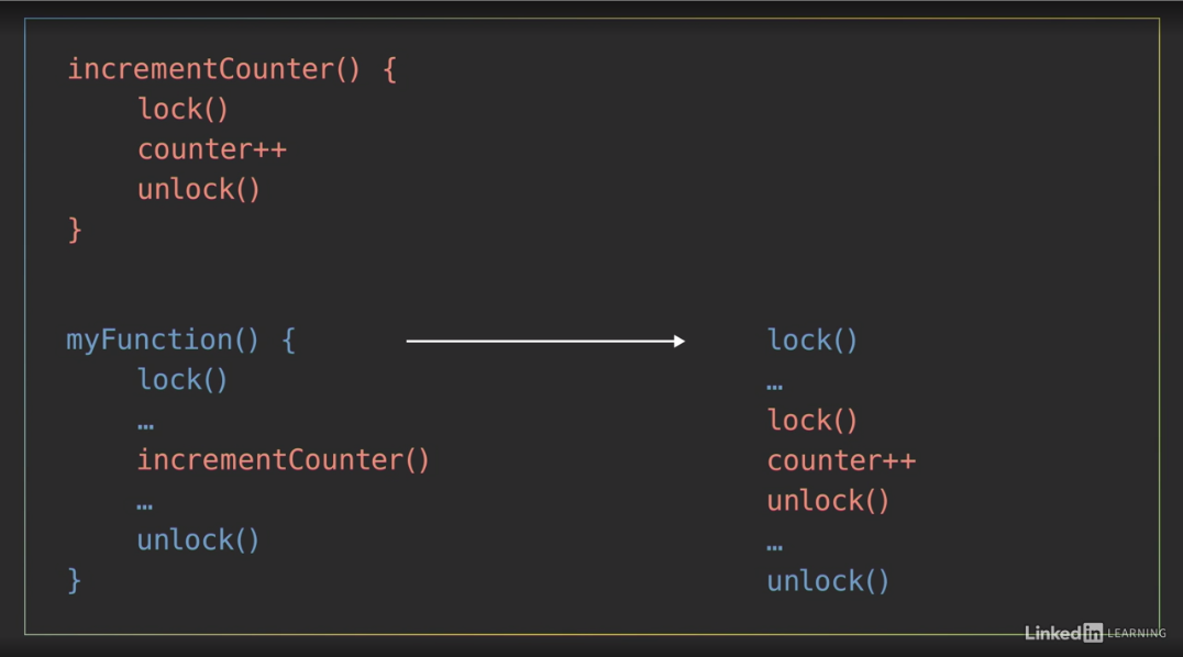
As an example, say I have a function to increment a shared counter, and it uses a mutex to protect that operation. If later I create another function that uses the same mutex to protect some other section of code, and that section of code uses the increment counter function, since those functions are nested, when I execute my function it will end up locking the mutex twice before unlocking it. If I was using a regular non-reentrant lock, that would produce a deadlock, but with a reentrant mutex this works just fine.

Like many things in the world of programmers, there are some very strong opinions about whether reentrant locks are good or evil. Some opponents of using reentrant locks will argue that the example I just showed you should be refactored to avoid having nested locks by using a third function that increments the counter and only gets called from within a protected section. I’m not going to advocate either way on this debate. There are pros and cons to both sides. -

One common use case of reentrant locks is in recursive function. If the function makes a recursive call to itself from within a locked section, it will lock the mutex multiple times as it repeats itself, and then unlock the mutex an equal number of times as it returns and unwinds.

Aliases: reentrant mutex = reentrant lock = recursive mutex = recursive lock

Reentrant lock: Java demo

In Java, there are three classes that implement the lock interface

• ReentrantLock
• ReentrantReadWriteLock.ReadLock
• ReentrantReadWriteLock.WriteLock

Java does not have a standard non-reentrant lock.

04_02

Demo lock and unlock on time

This is a variation of the previous example I used to demonstrate a data race and implementing mutual exclusion, with two shopper threads that concurrently increment the amount of items to buy on a shared shopping list. In this version, the shopper class has a private method on line 12 called addGarlic which uses the reentrant lock named Pencil to enforce mutual exclusion around a call to increment the class variable named Garlic on line 14. A related method on line 18 named addPotato performs a similar function to increment another class variable named potatoCount. Scrolling down, the shopper’s run method simply uses a for loop on line 25 to execute those addGarlic and addPotato methods 10,000 times each. Down in the program’s main method, I create and start two shopper threads and then after they finish running, I print out the amount of garlic and potatoes to buy. Running this program as is, indicates we need to buy 20,000 garlic and 20,000 potatoes, that’s quite a feast.

Demo lock/unlock more than once

Now let’s say every time I add a potato, I also want to add an additional garlic to my list because garlic and potatoes go really, really well together. To do that, I might add a call to the addGarlic method inside of the addPotato method immediately after I increment the potatoCount. By doing that, I’ve effectively nested multiple calls to lock the pencil. When the addPotato method gets called, it will lock the pencil on line 19. Then, when the addPotato method calls addGarlic two lines later, the addGarlic method will lock the pencil again on line 13. So, the pencil ends up being locked twice in a row by those nested methods, before then being unlocked twice as the nested methods complete. Fortunately, since I’m using a reentrant lock, this code runs just fine and it gives me the output that we should now buy 40,000 garlic and 20,000 potatoes.

Java actually has a method that allows us to view the number of times that a reentrant lock has been acquired: ReentrantLock.getHoldCount();

To use that, I’ll need to change the type of the pencil object on line 10 from the general lock interface to the more specific reentrant lock. Now, I’ll add a print statement to the addGarlic method right after locking the pencil to display the value of pencil.getHoldCount When I run this program, I see that the Hold count messages alternate between one and two. The Hold Count will be one for the times when the addGarlic method gets called directly and it will be two when the addGarlic method gets called from within the potato method and therefore the pencil gets locked twice.

Try lock

• non-blocking lock/acquire method for mutex
• if mutex available, lock it and return true
• if not, return false

When multiple threads each have multiple tasks to perform, making those threads block and wait every time they attempt to acquire a lock that’s already taken may not be necessary or efficient. Olivia and I are two threads doing several different tasks. My thread will be taking an inventory of the fridge to see what things we’re running low on and then add those to the shopping list on our shared notepad. I’ll go back and forth between those two tasks. - [Olivia] And my thread is searching through the newspaper for grocery coupons and then adding those items to the shared shopping list. Ooh, there are some good deals this week! Now that I’ve found some items that I want, I’ll take the pencil, which is our mutex, to lock access to the shared notepad so I can add them. - I saw we’re low on milk. So now I’ll go to acquire the pencil. And I see Olivia has it. If I attempt to lock a mutex in a regular blocking fashion, my thread would enter a waiting state at this point, doing nothing until Olivia unlocks it. If I don’t have anything else to do, so I can’t continue with other things until after I’ve accessed the shared notepad, that’s okay. It’s what has to happen, but in this scenario, I do have other useful things to do that don’t require the notepad. I can keep searching the fridge for other things we need. So, rather than using the standard locking method to acquire the mutex, I’ll use what’s called try lock, or try enter, which is a non-blocking version of the lock or acquire method. It returns immediately and one of two things will happen. If the mutex you’re trying to lock is available, it will get locked, and the method with return TRUE. Otherwise, if the mutex is already possessed by another thread, the try lock method will immediately return FALSE. That return value of true or false lets the thread know whether or not it was successful in acquiring the lock. So, if I try to lock the pencil that Olivia currently has, I know immediately that my attempt has failed. So I can go back to searching the fridge. - There, I’m done writing for now. So I’ll unlock the pencil and go back to searching for coupons. Since Barron wasn’t blocked waiting for this mutex, it’s just sitting unlocked available for anyone to take. Now, Barron likes to explain try lock with pencils and notepads. I think of it more like being at a house party with a bunch of your friends, your fellow threads. There’s one restroom at the house that everyone at the party will need to use at some point. But only person can use it at a time. When you try to use it, and try opening the door, you realize it’s locked because someone’s already inside. You could stand there and wait until they come out or you could go back to the party, keep having fun, and try again later.

Try lock: Java demo

This example demonstrates, with try lock, threads can become more efficient.

04_04

To demonstrate the try lock method in Java, I’ve created this example that simulates two shoppers searching for the items they need and then adding to a shared notepad. In this shopper class, each shopper has their own instance variable on line nine for the number of items they need to add to the notepad, which is how many items they found in a coupon book or perhaps missing from the fridge. The static integer on line 10 represents the number of items they’ve added to the shared notepad, and the pencil on line 11 is the lock that’s used to protect access to it. Down in the run method, the while loop on line 18 will keep the shoppers searching for items and adding them to the shared notepad until there are at least 20 items. If the shopper has items to add to the notepad, they’ll execute the if clause on line 19, in which they lock the pencil, add all of their items to the list, and then print a message with how many items they added. That then resets their items to add count back to zero. Their thread sleeps for 300 milliseconds, and then finally, it unlocks the pencil on line 29. If the shopper did not have anything to add, then they would have executed the else clause on line 31. Where they spend 100 milliseconds searching for an item that they need, which then increments their items to add count. Down in the main method, I create two shoppers named Barron and Olivia, then record the time from when I start their threads until they both finish to see how long it takes them both to find at least 20 items. Now I’ll run the program. And I see that it took them a little over six and a half seconds. Notice that their two threads are never adding more than one item at a time. Since the regular lock method blocks execution, these two threads end up taking turns, Swapping places between the top and bottom sections of that if else statement. Now, I’ll replace the standard lock method up on line 21 with Java’s try lock method. And, since the try lock method returns a Boolean value to indicate whether or not it successfully acquired the lock, I’m going to move and incorporate it into the if statement on line 19. Now, the order of these statements on each side of the and operator matters. Because Java evaluates statements from left to right. It will first check to see if there are any items to add, and only if the left side of the and operator is true will it evaluate the right side and execute that try lock method. If the lock is available, then calling try lock will acquire it and return true. So the program will execute the code between lines 20 to 29 to add items to the shared notepad. If the lock was not available, then since try lock doesn’t block execution, it will immediately return false. And that thread will execute the else clause from lines 31 to 37 to look for other things to buy. When I run the program now, it executes much faster, finishing in under two and a half seconds, which is less that half the amount of time as before. Notice that now, when one of the threads gets its turn in the critical section, it’s often adding more than one item to the notepad. With the try lock method in place, as one thread takes its time writing to the notepad, the other thread is able to jump past that section of code to search for other things to buy multiple times. That thread has been freed up to accomplish other useful things.

Read-write lock

The generic locker mutex locks the resource no matter the operation, while if it’s only read operation, we don’t necessarily need to lock the data. Write operation is where locking is needed.

A reader-writer lock or shared mutex can be locked in one of two ways

• shared read mode that allows multiple threads read simultaneously
• exclusive write mode that limits access to only one thread to safely write.

An example

A read-write lock is useful for protecting a shared resource like our calendar, because Baron and I frequently need to read the calendar throughout the day. - I can never remember what day it is. - But we rarely need to modify it. - Once once a day. - This marker represents our shared mutex. When my thread wants to read the calendar, I’ll lock the mutex in the read only mode by placing my finger on it. - I also want to read the calendar, I can also place my finger on the marker. Now we both have a shared lock on it, so we can both concurrently read it. - When I’m done checking the date, I’ll release my lock on the mutex. Now, I think it’s time to increment the calendar’s date. In other words, I want to modify it, and to do that, I’ll need to lock the shared mutex in exclusive write mode by picking it up. - But I’m still holding onto the lock to read. - A thread trying to acquire the lock in write mode can’t do so as long as it’s still being held by any other threads in the read mode, so I’ll have to wait. - Done. - Now the shared mutex is completely free, so I’ll pick it up to place a write lock on it and update the calendar. - Ah. I already forgot what day it is. And I can’t read the calendar now because Olivia has an exclusive hold on the lock to write. Since only one thread can have the write lock at a time, all other threads wanting to read or write will have to until the lock becomes available again.

When to use a read-write lock

• In certain scenarios, read-write locks can improve a program’s performance versus using a standard mutex.
• more complicated to implement
• typically use more resources under the hood to keep track of the number of readers
• there can be language dependent differences in how they’re implemented that affect performance
  • e.g. Do they give preference to readers, or writers that are trying to acquire the lock?

A general rule of thumb:

• Use a shared reader-writer lock when # of read threads > # of write threads. such as certain types of database applications.
• If the majority threads are writing, then there’s not much advantage to using a read-write lock.

Read-write lock: Java demo

04_06

    private static ReentrantLock marker = new ReentrantLock();
    ...
    marker.lock();
    marker.unlock();

    private static ReentrantReadWriteLock marker = new ReentrantReadWriteLock();
    private static Lock readMarker = marker.readLock();
    private static Lock writeMarker = marker.writeLock();
    ...
    writeMarker.lock();
    writeMarker.unlock();
    readMarker.lock();
    readMarker.unlock();

5. Liveness

Deadlock

Dining philosophers problem:

• each philosopher need to pick up both chopsticks to eat
• picking up the two chopsticks happens in two steps
• possible scenario is two philosophers each pick up one chopstick, and waits on the other chopstick
• deadlock
• Set priorities to chopsticks can solve it

Deadlock: Each member is waiting for some other member to take action, and as a result, neither member is able to make progress.

Avoiding deadlock is common challenge in concurrent programs that use mutual exclusion mechanisms to protect critical sections of code.

Deadlock to liveness, which is

• a set of properties that require concurrent programs to make progress
• Some processes or threads may have to take turns in a critical section A well-written program with liveness guarantees that all processes will eventually make progress.

A realistic scenario:

imagine something like a banking application with a set of bank accounts where each one has its own mutex to ensure that only one thread will be withdrawing from or depositing funds to that account at time. To transfer funds between two accounts, a thread needs to acquire the locks for both the sender and the receiver since it would be modifying the value of both accounts. If there are multiple threads concurrently making transfer between the accounts, then there’s a real chance that they could end up competing for the same locks and run into this sort of deadlock scenario.

Deadlock: Java demo

And this highlights the tricky nature of Deadlocks and why they can be hard to detect and debug. Just like Data Races, you might get lucky and never have your program lock up, even if the potential for a Deadlock exists.

Potential fixes for deadlock:

• Lock ordering:
  • may not always be feasible. For example, a thread may not know all of the locks it will need to acquire ahead of taking any of them.
• locking timeout: Put a timeout on lock attempts, if a thread is not able to successfully acquire all of the locks it needs within a certain amount of time it will:
  • back up, free all of the locks taken
  • wait for a random amount of time
  • try again

Abandoned lock

Now that we figured out how to avoid a deadlock between our two philosophers using chopsticks, we can return to our routine of eating and philosophizing. I’m ready for another piece of sushi so I’ll pick up the first chopstick, then the second one. And I think I left the refrigerator open. - Oh, that was rude of him.

We’ve entered another form of a deadlock through thread death. If one thread or process acquires a lock, and then terminates because of some unexpected reason, it may not automatically release the lock before it disappears.

That leaves other tasks like me stuck waiting for a lock that will never be released and getting hungry. - Sorry about that. Let’s look at some code.

Abandoned lock: Java demo

To demonstrate what happens if you abandon a lock in Java, I’ll be modifying a version of the previous dining philosophers example that I used to demonstrate a deadlock. It has three philosophers using chopsticks to take sushi from a shared plate. I’ve already fixed the deadlock in this version, so if I run this program, the philosophers successfully take turns eating sushi until all of the pieces are gone.

The critical section for this program exists between the lock calls on line 23 and 23, and the calls to the unlock method on lines 32 and 33. Now, if one of the philosopher threads acquires those locks and then something goes wrong in the critical section and throws an unexpected error, that could cause its thread to terminate before it gets a chance to release those locks. To simulate that happening, I’m going to add another if statement that checks to see if there are exactly 10 pieces of sushi left. And if so, I’ll use my favorite technique for intentionally crashing a thread, dividing by zero. Now, you should never intentionally divide by zero, but I’m doing it here to throw an exception that will cause Java to crash one of these threads. When I run this program, it gets all the way down to 10 pieces remaining. Then, the thread that happens to be executing at that time hits the divide by zero case, and crashes. In this run, Olivia was the unlucky thread. The other two threads are stuck waiting on the locks that Olivia will never release, so the program is stuck here forever.

This scenario is slightly different than the deadlock we looked at previously because the threads are not waiting on each other to release the lock. But it’s a related scenario and the impact is the same. This program isn’t making any progress.

So, to prevent this type of situation from occurring in Java, I should wrap the critical section in a try block. If I want, I can include any exception handling code in a catch statement after that. But what I really care about here is making sure that the locks always get released. And to do that, I’ll add a finally block after the try statement, and I’ll move the calls to unlock the chopsticks into it. Now when I run the program, an exception still occurs when Barron takes the 10th remaining piece of sushi, but thanks to the finally clause, Barron’s thread is able to release the lock before terminating. I can see that after the 10th item, Olivia’s thread took over to finish eating the rest of the sushi.

This is a good practice to follow when using locks in Java. Always put the critical section in a try block and release the locks in a finally clause just in case something goes wrong.

Starvation

Starvation: a process or thread is unable to gain access to a necessary resource (i.e. perpetually denied the resources it needs), and is therefore unable to make progress. If another greedy thread is frequently holding a lock on the shared resource, then the starved thread won’t get a chance to execute.

Two main causes of starvation

• Lower priority threads doesn’t get to be scheduled
• Too many concurrent threads

It would be nice if Olivia and I took turns acquiring and releasing the pair of chopsticks so we could each take an equal amount of sushi from the shared plate. But that’s not guaranteed to happen. The operating system decides when each of our threads gets scheduled to execute, and depending on the timing of that, it can lead to problems. If Olivia puts down the chopsticks to release her lock on the critical section, but my thread doesn’t get a chance to acquire them before she takes them again, then I’ll be stuck waiting again, until she takes another piece. If that happens occasionally, it’s probably not a big deal. But if it happens regularly. - Too slow. - Then my thread’s going to starve.

In a simple scenario like ours, with two equal threads competing for execution time, starvation probably isn’t a concern. Both of our threads should get plenty of chances to take sushi. However, if our two threads are given different priorities, then that may not be the case. Baron knows I can get grumpy when I don’t eat. - And I certainly don’t want that, so I’ll give Olivia’s thread a higher priority. - Thanks. - How different thread priorities get treated will depend on the operating system. But, generally, higher priority threads will be scheduled to execute more often and that can leave low priority threads like me feeling hungry.

Another thing that can lead to starvation is having too many concurrent threads. - Oh, I forgot to mention that I invited some friends over. (scoffs) - Well, with this many competing threads, I may never get any sushi.

Starvation: Java demo

To demonstrate thread starvation in Java, I’ll modify the dining philosophers example program by adding a local variable within the philosophers classes run method to keep track of the number of pieces of sushi, this philosopher thread gets to eat. I’ll increment that sushi eaten variable every time the philosopher takes a piece of sushi. And finally at the end of the run method after the while loop finishes, I’ll print out the number of pieces that this philosopher was able to take. When I run this program… I see that each philosopher got a different amount of sushi and it’s not particularly fair. Olivia took way more sushi than Barron or Steve here, but that’s not because she is greedy, it’s because of the order in which three philosophers are currently taking chopsticks. Barron and Steve and both competing for chopstick A as their first chopstick, but Olivia is the only philosopher going for chopstick B first. So since she has less competition to get her first chopstick, she ends up being able to take sushi more frequently. So to make things fair here, I’ll make all of the philosophers acquire the same two chopsticks A and then B. And then I’ll run the program again. And now they end up with a much more even and fair distribution. With half a million of sushi, there is plenty to go around so all of these philosophers are well fed.

Now let’s see what happens if I drastically increase the number of philosophers at this dinner party by using a for loop to create 5,000 instances of Barrons, Olivias and Steves, which means 15,000 total philosophers will be competing for just half a million pieces of sushi. Now, after running this program… As I scroll through the final counts for each thread, I can see that some of the philosophers got a lot of sushi compared to others and many philosophers starved completely.

All of these threads were created with the same default priority but because there were so many of them, some of the threads never got a chance to execute, and this represents a real problem in programs containing huge numbers of threads. For example, if instead of feeding sushi to a bunch of philosophers, this program was web server that created new threads to handle a huge number of incoming requests, some of those requests may never get processed, and that would lead to some impatient and angry users on the other end. There are techniques that can be used to improve or even guarantee fairness among threads, but that type of word cloud management is very situation dependent and beyond the scope of this course.

Livelock

livelock: multiple threads or processes are actively responding to each other to resolve conflict, but that prevents them from making progress, could be solved by priority, random selection, etc.

Our greed and competition for sushi has led us to a life of deadlocks and starvation. There’s only one piece of sushi left and I can see you’re still hungry, you should have it. - Thank you my dear, but I can see you’re still hungry too. And I would feel like a lousy husband if I allowed my wife to go hungry. You should have the last bite. - Oh but I can’t bear to see you hungry, you shall have the final bite. - Well this is annoying. We’ve entered into another tricky situation known as a livelock.

A livelock looks similar to a deadlock in the sense that two threads are blocking each other from making progress, but the difference is that the threads in a livelock are actively trying to resolve the problem.

A livelock can occur when two or more threads are designed to respond to the actions of each other. Both threads are busy doing something, but the combination of their efforts prevent them from actually making progress and accomplishing anything useful. The program will never reach the end.

The ironic thing about livelocks is that they’re often caused by algorithms that are intended to detect and recover from deadlock. If one or more processor thread takes action to resolve the deadlock, then those threads can end up being overly polite and stuck in a livelock. To avoid that, ensure that only one process takes action chosen by priority or some other mechanism, like random selection. - Rock, paper, scissors for it? - One, two, three, shoot. - I win! - Now Olivia gets the last piece of sushi and that resolves our livelock.

Livelock: Java demo

To demonstrate a livelock in Java, I’ll modify the dining philosophers example from earlier that I used to demonstrate a deadlock. Now, I have not implemented a strategy to prevent the deadlock in this version, so if I run this program, sure enough, after a few iterations, it hits a deadlock. The philosophers have acquired their first chopstick lock, and they’re stuck waiting for their second one to become available. One possible way to fix this problem would be to have the philosophers release their lock on their first chopstick if their second chopstick is not available when they try to take it. That will give another philosopher a chance to take that first chopstick and hopefully prevent the deadlock. To implement that, instead of using the regular lock method, on the second chopstick, I’ll use the TryLock method on it. And, I’ll put that in an if statement that will execute if the lock was not taken. If that happens, I’ll print a message that this philosopher released their first chopstick and then release it. (keyboard typing) Otherwise, in the corresponding else clause, I’ll continue on as normal with the run method. That should prevent a deadlock, so I’ll run the program, and I just see a lot of messages that the philosophers are releasing their first chopstick. Occasionally, the scheduling works out so that one of these philosophers is able to acquire both of the locks they need to take a bite of sushi, so this is not a complete livelock scenario, but the majority of the time, these philosophers are picking up their first chopstick and then politely putting it back because another philosopher probably needs it. If I press ctrl+shift+esc to bring up the Windows Task Manager and look at the Performance tab, I see that the CPU is being pretty steadily utilized. All of those threads are actively working to pick up and put down their chopsticks. They’re just not making any progress towards the end of the program.

Livelocks can be even harder to locate and debug than deadlocks, but when you’re multithreaded program seems to be stuck in some sort of lock, looking at the CPU utilization may give you some insight into whether it’s a livelock or a deadlock. This program’s going to keep running for a long time, so I’ll stop it by clicking the stop button in IntelliJ

To resolve this livelock, I’m going to introduce some randomness by importing the Java.util.Random class. (keyboard typing) Then I’ll give the philosopher class its own random object, which I’m going to call RPS, which stands for Rock, Paper, Scissors. And finally, after a philosopher decides to put back their first chopstick, I’ll make them sleep or philosophize for a random amount of time before they try taking their first chopstick again. (keyboard typing) And since that sleep statement can throw an exception, I’ll need to wrap it in a try catch clause. IntelliJ makes that easy with a little red lightbulb. Now when I run the program one final time, I see way fewer instances of the philosophers returning their chopsticks, so they’re able to keep taking pieces of sushi. The program makes progress, and it’s able to finish without running into a deadlock.

Thread.sleep() may throw exception, so try catch is necessary

Parallel and Concurrent Programming with Java 2

Intro

1.Synchronization

Condition variable

Baron and I just made a slow cooker full of delicious hot soup and I’m ready to dig in. - But we should take turns to make sure we each get our fair share of soup. In this scenario, we’re two hungry threads competing for access to a shared resource, the soup, and the slow cooker lid will act as a mutex to protect it. Only the thread that holds the lid can check to see how much soup is left, determine if it’s their turn to take the next serving and modify the amount of soup that’s left by taking some. - Hmm, that was some really good soup. I think I’ll have another serving. Oh, I see you haven’t taken your share yet. What about now? How about now? Now? - Olivia’s thread is wasting a lot of energy repeatedly acquiring the mutex to check for a certain condition, to see if her turn to take more soup, and she’ll continue doing that until my thread eventually gets scheduled, so I can acquire the lid, see that it’s my turn and take my serving. - What I was doing is called busy waiting or spinning,

Busy waiting, aka. spinning: repeatedly acquiring and releasing the lock to check for a certain condition to continue. It isn’t very efficient, especially if it goes on for a long time.

This is one of the limitations of using just a mutex.

• Sure, it restricts multiple threads from taking soup at the same time
• but the mutex alone doesn’t give our threads a way to signal each other to synchronize our actions. To do that, we can use another mechanism called a condition variable

Condition variable: a queue or container for threads that are waiting for a certain condition to occur. Think of it as a place for threads to wait and be notified.

The condition variable is associated with a mutex. The condition variable + a mutexthey = a monitor, a higher level construct.

Monitors

• protect a critical section of code with mutual exclusion
• provide the ability for threads to wait/block until a certain condition occurs, and signal those waiting threads

Conceptually

• A monitor: a room that contains the procedures and shared data that you want to protect. Only one thread can be in that room at a time to use those procedures and access the data.
• Mutex: a lock on the door.
• condition variable: waiting room.
  • Other threads that try to enter the protective section while it’s occupied will wait outside in a condition variable/waiting room.
  • There might be multiple condition variables or multiple waiting rooms, waiting for different conditions to occur to acquire that same mutex.

• When the thread inside the monitor finishes its business in the critical section
  • it will signal one of the conditions that it’s their turn to execute
  • then it releases its lock on the door to exit the critical section.
• One of the threads waiting for that condition that was signaled will
  • wake up
  • take its turn in the monitor
  • locking the door behind it, execute the critical section

Now, the condition variable has three main operations.

• wait:
  • Before using a condition variable, the thread acquires the mutax, check the condition, and the condition doesn’t meet
  • automatically release lock on the mutex
  • go to sleep and enter waiting queue
  • reacquire lock when woken up
• signal
  • wake up one thread from condition variable queue
  • called signal, notify, wake depending on language
  • release lock on mutex
• broadcast
  • wake up all threads from condition variable queue
  • may be called notifyAll or wakeAll

Before using a condition variable, I first need to acquire the mutex associated with it, check for my condition, I see that it’s not my turn to take more soup, so I’ll use the condition variable’s wait operation, which releases my lock on the mutex and then puts my thread to sleep or a pause state and places it into a queue waiting for another thread to signal that somebody else takes the soup.

Since Baron released his lock on the lid before going to sleep, now I can acquire it, see that it’s my turn to take some soup, so I’ll do that. Then, I’ll use the signal operation to wake up a single thread from the waiting queue, so it can acquire the lock. Depending on the language you’re using, you will also see this operation called notify or wake. Baron, wake up, it’s your turn to take some soup. Finally, I’ll release my lock on the mutex. - Ah, my turn. The third condition variable operation, broadcast, is similar to the signal operation except that it wakes up all of the threads in the waiting queue. You may also see it called things like notify all or wake call.

Now, in this little scenario, we only had two threads signaling each other on a single condition, that somebody took soup which then changes whose turn it is to take the next serving.

implementing a shared queue or buffer

• mutex
• condition variables
  • bufferNotFull: for threads adding item
  • bufferNotEmpty: for threads taking item

A more common use case that requires multiple condition variables is implementing a shared queue or buffer. If multiple threads will be putting items in a queue and taking them out, then it needs a mutex to ensure that only one thread can add or remove items from it at a time, and for that, we can use two condition variables. If a thread tries to add an item to the queue, which is already full, then it can wait on a condition variable to indicate when the buffer is not full. And if a thread tries to take an item but the queue’s empty, then it can wait on another condition variable for BufferNotEmpty. These condition variables enable threads to signal each other when the state of the queue changes.

Condition variable: Java demo

01_02

This Java program, to demonstrate using condition variables, defines a class named HungryPerson on line seven, which has three variables, an instance variable named personID on line nine, which is a unique ID number that gets passed to the HungryPerson constructor method, a static class variable named slowCookerLid, which is the reentrant lock that protects access to the third variable on line 11, representing the number of servings in the slow cooker, which gets initialized to 11. When a HungryPerson thread starts, the run method uses a while loop on line 18 to keep taking servings of soup until there’s none left. For each iteration of the loop, the HungryPerson takes the slowCookerLid by locking it on line 19, then they check to see if it’s their turn to take the next serving by comparing their ID number to the number of servings left, modulo two since there are two people in this example. If it is their turn, and there’s soup left in the pot, then they take a serving of soup by decrementing the shared servings value on line 22 and print a message that includes how much soup is left. If it was not their turn, then they print a message about putting the lid back, and then finally, on line 30, the thread unlocks the slowCookerLid for another HungryPerson to take. Down in the main method, I simply use a for loop on line 38 to create and start two HungryPeople to eat soup. If I run this program I see that these two threads spend a lot of cycles checking to see if it was their turn and then putting the pot lid back. If I scroll up through the output I see that over the course of all that, the two threads do take turns eating, and it’s just not very efficient.

So let’s use a condition variable for them to communicate. I’ll add a static condition object to the HungryPerson class to signal after one of the threads has taken soup. And I’ll associate that condition variable with the slowCookerLid by creating it with a newCondition method on that object. The basic usage pattern for a condition variable involves locking the mutex, then using a while loop to check if the condition we’re looking for is true. If it’s not true, then we’ll wait on the condition variable for another loop iteration. Otherwise, when the condition is true, we’ll continue past the loop to execute the critical section of code and then finally release the lock. Now, I want to emphasize here that the conditionVariable is not the condition itself or an event. The condition that we’re checking for is the logic of the while loop. Is it this thread’s turn to take soup? The conditionVariable is just a place for threads to wait until they’re signaled by another thread. To implement that in this program, I’m going to turn the if statement on line 22, that checks to see if it’s that person’s turn, into a while loop that checks to see if it’s not their turn. If it’s not this thread’s turn then it uses the soupTaken condition variables await method to release its hold on the slowCookerLid and wait until it gets signaled. I’ll also move the print statement about the thread putting the lid back into this loop. And I’ll clean things up after making those changes by deleting the empty else clause. Now, the basic pattern for signaling a condition variable involves first making sure you have a lock on the mutex, to ensure you have exclusive access to whatever comprises the condition. Then doing something that changes the state for that condition, signaling at least one of the other waiting threads to wake up, and finally, unlocking the mutex so another thread can proceed to use it. In this example, the HungryPerson takes ownership of the SlowCookerLid lock on line 20, and they will reacquire a lock on it whenever waking up from the await statement on line 24. When a thread decrements the servings variable, that’s what changes whose turn it is next. So I’ll use the ConditionVariable’s signal method after that to let another waiting thread know it should wake up and check if it’s their turn to take soup. Now I’ll run the program and I see that the two HungryPeople take turns. And they don’t waste a lot of energy repeatingly checking whose turn it is, although they did continue to take soup after it was all gone, so we ended up with negative servings. To fix that I’ll wrap the lines that involved taking soup in an if statement to only execute if there are servings left to take. Now I’ll run it again, and fixed. We end up with zero servings at the end. Now, let’s see what happens if we expand this dinner party to include more HungryPeople by modifying the for loop in the program’s main method to create five HungryPeople threads. And I’ll also modify the condition statement on line 22 to rotate servings among those five people. Now I’ll run the program again, and this time it gets stuck. The problem here is that I used the signal method, which will only wake up one of the waiting threads. If it doesn’t wake up the correct thread, whose turn it is next, then the program will get stuck. So, I’ll close the console to terminate this program, and the fix here is to change that method on line 29 to signal all, to notify all of the waiting threads to wake up and check that it’s their turn. Now when I run the program, everything works great. All of the threads eat and they take turns signaling each other to do so.

If you only need to notify one of the waiting threads, and you don’t care which one it is, then the basic signal method works fine. But in this example, since I wanted a specific thread to wake up and see that it’s their turn, relying on the signal method to wake up the right thread will lead to the program getting stuck.

Using a conditiona variable

• acquire the mutex first
• check if some contiiton is not true, wait for signal
• once signaled, condition matches, execute critical section
• release mutex ``` mutex.lock(); while (some condition not true) {//The condition conditionVariable.await();//wait here until signaled }

//Execute critical section.

mutex.unlock();

#### Signaling a Condition Variable
* acquire the mutex first
* do something and change the contition
* signal
* release mutex

mutex.lock(); //Do something that chagnes state of condition conditionVariable.signal(); mutex.unlock();

### Producer–consumer
A common design pattern in concurrent programming is the producer-consumer architecture where one or more threads or processes act as a producer which adds elements to some shared data structure and one or more other threads act as a consumer which removes items from that structure and does something with them. 

> To demonstrate that, I'll be the producer serving up bowls of soup. - I guess that makes me the consumer who eats the soup. I like this demonstration. - After I fill a bowl, I'll add it to this line of bowls that represents a queue. *Queues operate on a principle called a First-In-First-Out or FIFO which means items are removed in the same order that they're put into the queue.* The first item that was added will be the first item to be removed. - So when I'm ready to consume another bowl of soup, I'll grab one from this end of the line because it's been in the queue the longest. These bowls of soup represent elements of data for the consumer thread to process or perhaps packaged tasks for the consumer to execute. 

When multiple threads are operating in this type of producer-consumer situation, it poses several challenges for synchronization. 
* First off, the queue is a shared resource, so we'll need something to enforce mutual exclusion and make sure that only one thread can use it at a time to add or remove items. 
* We also need to make sure that the producer will not try to add data to the queue when it's full. 
* And that the consumer won't try to remove data from an empty buffer.

Some programming languages may include implementations of a queue, that's considered thread safe, and handles all of these challenges under the hood so you don't have to but if your language does not include that support, then you an use the combination of a mutex and condition variables to implement your own thread-safe synchronized queue.

> (slurping) Hey, Olivia, you can slow down production. I can't eat soup this fast. - No can do, I'm a soup serving machine.

#### Rate of consumer vs producer
You may run into scenarios where the producer cannot be paused if the queue fills up. The producer might be an external source of streaming data that you can't slow down so **it's important to consider the rate at which items are produced and consumed from the queue**. **If the consumer can't keep up with production, then we face a buffer overflow and we'll lose data.** 

> This table is only so big, our queue can only hold a limited number of bowls of soup before they start falling on the floor. 

**Unbounded queues**(in some langs): are implemented using linked lists to have an advertised **unlimited capacity** but keep in mind, even those will be **limited by the amount of physical memory in the computer**

The rate at which the producer is adding items may not always be consistent. 
> For example, in network applications, data might arrive in bursts of network packets which fill the queue quickly but if those bursts occur rather infrequently, the consumer has time to catch up between bursts. 
You should consider the **average rate** at which items are produced and consumed. You want the **average rate of production to be less than the average rate of consumption**.

> Well, it looks like you're pouring at a pretty steady pace and I definitely can't keep up alone. I'm going to need some help. Hey Steve, do you want some soup? - You bet, my friend, I'm a soup eating machine. - Excellent. With two consumer threads eating in parallel, maybe we'll be able to keep up with Olivia's rate of production. Now there are only two tasks going on here. Olivia is serving soup while Steve and I eat it. But if more steps were required to process this data, perhaps we also need to season the soup, then we could expand our simple producer-consumer setup into a pipeline of tasks. 

#### Simple producer-consumer setup can expand into a pipeline of tasks. 

![Pipeline.png]()

A pipeline consist of a chain of processing elements arranged so that the output of each element is the input to the next one. It's basically a series of producer-consumer pairs connected together with some sort of buffer like a queue between each consecutive element.
> As a pipeline, I pass my full bowls of soup to a queue. - I take bowls from that queue, add spice, then I pass them along to another queue which Steve takes from to eat. If all three of our threads can execute in parallel, then as a pipeline, we're processing up to three bowls at any given moment. Now the issue of processing rates is still a concern. **Each element needs to be able to consume and process data faster than the elements upstream can produce it.**

### Producer–consumer: Java demo

01_04

`ArrayBlockingQueue<E>` a bounded queue, implements `BlockingQueue<E>`, uses an Array.
`BlockingQueue<E>` is thread safe, noneed for manually adding mutex.

* `ArrayBlockingQueue<E>.add()`
* `ArrayBlockingQueue<E>.take()`

> This Java example has two primary classes which I currently have hidden using code folding. A SoupProducer class on line 7, and a soupConsumer class that begins on line 26. Down in the program's main method on line 47, I instantiate a blocking queue named servingLine which will be used to pass bowls of soup from producers to consumers. It's a fixed length array blocking cube which has the capacity to hold up to five string objects. I use constructor methods on lines 48 and 49 to create and start soupProducer and consumer threads, both of which take the queue as an input argument. Java's ArrayBlockingQueue is a concrete class that implements the blocking queue interface. It's a bounded queue that uses an array under the hood to hold a finite number of elements. An important thing to note about the ArrayBlockingQueue is that since it implements the blocking queue interface, it's thread safe, meaning it already has mechanisms in place to prevent multiple threads from improperly accessing it, and potentially causing a data race. So, thanks to Java, we conveniently don't need to include any locks in this example to protect the queue. Looking inside the soupProducer class, the run method uses a for loop on line 16 to serve 20 bowls of delicious hot soup. For every iteration, it tries to add a string object that represents a bowl of soup to the serving line. If there is space available in the queue then the the add method will insert the item. Otherwise, it'll throw an exception. After that, the producer prints a message on line 19 that it served a bowl along with the number of remaining spaces in the queue, and finally, on line 20, it sleeps for 200 milliseconds to simulate the time it takes to serve a bowl of soup. Now, down in the soupConsumer's run method, the while loop on line 35 will make the consumer thread continuously take and eat soup from the serving line forever. It calls the queues take method on line 37. To get the string representing a bowl of soup, it prints a message that it ate that bowl, and then, on line 39, the consumer sleeps for 300 milliseconds to simulate the time it takes to eat soup. Those are all the pieces. So, now, I'll run this program, and I see messages from the producer that it's serving bowls of soup, and from the consumer, that it's eating them. However, after a while, the soup producer throws several errors that the queue is full before it ends, and then, the consumer finishes the remaining bowls that were already placed in the queue. The problem here is that the producer is adding soup faster than the consumer can eat it. It only takes 200 milliseconds to produce a bowl of soup, but 300 milliseconds to consume it. Scrolling back up through the output, I see that the remaining capacity of the serving line gradually decreased from five down to zero before the producer threw errors. To solve this problem, I'll add a second consumer thread to this program to help eat soup. Although it takes each soup consumer 300 milliseconds to eat a bowl, now that I have two of them working together, the throughput of my program increases, so it can process a bowl every 150 milliseconds which is faster than the soupProducer serves it up. So, when I run the program now, the consumers are able to keep up with the producer, and everything works fine, except that this program never finishes running because the consumer threads are still running, waiting for more soup to come down the serving line for them to eat. So, I need to implement some sort of signal for the consumers that the producer is done, and one way to do that is to pass a final message through the queue. After the soupProducer's for loop completes, I'll add a final string to the queue with a special message for the consumer, no soup for you, and since there are two consumers, I'll need to add that twice, once for each. Now, down in the soupConsumer, after retrieving a string from the queue, I'll check to see if it says no soup for you, and if so, I'll break out of the while loop. Now, when I run this program, all of the soup gets eaten, and it finishes appropriately. I used strings to represent bowls of soup in this example, but queues can be used to pass other types of data, or other packaged tasks for the consumer thread to process.

### Semaphore
* sync mechanism
* allows multiple threads to use
* include a counter to track availability

#### Operation `acquire()`
* if counter > 0, decrement counter
* if counter == 0, **wait** until it's available

#### Operation `release()`
* release semaphore, and increment counter
* signal waitting threads

A semaphore is another synchronization mechanism that can be used to control access to shared resources, sort of like a mutex, but unlike a mutex, a semaphore can allow multiple threads to access the resource at the same time, and it includes a counter to track how many times it's been acquired or released. As long as the semaphore's count value is positive, any thread can acquire the semaphore, which then decrements that counter value. If the counter reaches zero, then threads trying to acquire the semaphore will be blocked and placed in a queue to wait until it's available. When a thread is done using the resource, it releases the semaphore, which increments that counter value and if there are any other threads waiting to acquire the semaphore, they'll be signaled to wake up and do so. 

#### Example
> Hmm, looks like my phone's about to die. - Lucky us. There is a charger right here. - Nice, this charger has two ports. So it can be used by up to two devices at the same time. You can think of the number of open ports as a semaphore. Right now, this semaphore has a value of two, because there are two free ports. And when I acquire one of these ports by plugging in my phone, it decrements the semaphore's value to one. - I'll acquire the other port. And that decreases the semaphore's value to zero, which means it's unavailable for anyone else to use. - Lucky me, there's a charger right here. - Oh man, sorry Steve. The semaphore's locked right now because there aren't any available ports. You'll have to wait until one of us is done charging and releases the semaphore. - No worries, I'll wait. - You know, I don't need to charge that bad. I'll release my port, which increments the semaphore's value and I'll notify Steve that it's available. Hey Steve, wake up. - Cool, now the semaphore's positive, I can acquire it and charge my phone.

#### Counting semaphore
* value >= 0
* used to track limited resources
    - pool of connections
    - items in a queue

This type of semaphore that we're using here is called a counting semaphore, because it can have a value of zero, one, two, three, and so on, to represent the number of resources we have. In our scenario, we're counting available charger ports but in software, a counting semaphore might be used to manage access among multiple threads to a limited pool of connections for something like a server or a database. Or a counting semaphore could be used to track how many items are in a queue. 

#### Binary Semaphore
* value = 0 or 1
    - 0 locked
    - 1 unlocked
* similar to mutex by acquiring and releasing
* different from mutex
    - mutex need to be acquired/released by **same** thread
    - semaphore can be acquired/released by **different** threads


That may sound like a recipe for trouble and it certainly can be if you're not careful, but the ability for different threads to increment and decrement a semaphore's value and for threads to wait and be signaled by the semaphore is what enables it to be used as a **signaling mechanism**, to synchronize the action between threads. 

For example, a pair of semaphores can be used in a similar way to condition variables to synchronize producer and consumer threads, adding and removing elements from a shared, finite queue or buffer. One semaphore tracks the number of items in the buffer, shown here as fillCount, and the other one tracks the number of free spaces, which I'll call emptyCount. To add an element to the buffer, the producer will first acquire the emptyCount, which decrements its value, then it pushes the item into the buffer and finally it releases the fillCount semaphore to increment its value. Now, on the other side of the buffer, when the consumer wants to take an item, it first acquires fillCount to decrement its value, then it removes an item from the buffer and finally increments the emptyCount by releasing it. Notice that the producer and consumer each acquire a different semaphore as the first operation in their respective sequences. If the consumer tries to take an item when the buffer is empty, then when it tries to acquire that fillCount semaphore, it'll block and wait until a producer adds an item and releases fillCount, which will then signal the consumer to continue. Likewise, if the producer tries to add an item to the fillBuffer, then it goes to acquire the the emptyCount semaphore. It'll block and wait until a consumer removes an item and releases the emptyCount.

![Producer-Consumer Semaphore.png]()


### Semaphore: Java demo
01_06

For this Java example, I'll use a counting semaphore to control access and keep track of the number of available ports on a cell phone charger. This class named CellPhone has a static semaphore variable named charger on line nine, which I've initialized to have a value of four, representing the number of charger ports available to connect to. In the cell phone's run method, it will try to acquire the semaphore on line 17. If the semaphore is not available because its value is zero, then the thread will wait there until a charging port opens up and the semaphore is released. Once a cell phone thread has acquired the semaphore, it prints a message that it's charging and then sleeps for a random amount of time from one to two seconds. After that, the cell phone will execute the finally clause on line 22, which prints a message that it's done charging and then releases the semaphore to increment its value so another thread can acquire it. Down in the main method, I just use a for loop to create and start 10 cell phone threads on line 32. When I run this program, I see four of the phones connect immediately at the beginning, and then as each phone finishes charging and releases the semaphore, another phone acquires it to begin charging. At most, there will be four phones connected to this charger at any given time. Instead of using it as a counting semaphore, if I change the initialization value for the semaphore from four to just one, it'll act as a binary semaphore. When I run this program again, now only one thread at a time will be able to acquire the semaphore. The way I'm using the binary semaphore in this example, with the same thread that acquires it also releasing it, means it's basically acting the same as a mutex. In fact, I could replace all of the semaphore code in this particular program with re-entrant locks and it would function the same way.
## 2. Barriers
### Race condition

#### Data race vs race condition
* Data race: critical section is not protected
* Race condition: the order of execution is not deterministic, resulting in inconsistent results


<!-- Simplify following lines -->
Data races and race conditions are two different potential problems in concurrent programs that people often confuse with each other probably because they have similar sounding names with the word race in them. 
* Data races can occur when two or more threads concurrently access the same memory location. If at least one of those threads is writing to or changing that memory value, that can cause the threads to overwrite each other or read wrong values. - That's a pretty straightforward definition, which makes it possible to create automated tools to identify potential data races in code, and to prevent those data races, you need to ensure mutual exclusion for the shared resource.
* A race condition, on the other hand, is a flaw in the timing or ordering of a program's execution that causes incorrect behavior. 

In practice, many race conditions are caused by data races, and many data races lead to race conditions, but **those two problems are not dependent on each other.**

It's possible to have data races without a race condition and race conditions without a data race. 

#### Example
> Olivia and I invited Steve and the gang over to play video games next weekend, so we need to figure out how many bags of chips we need to buy to keep them all fed. Our shopping list is the shared resource, and this pencil serves as a mutex to protect it. Only the person or thread with the pencil can view or modify the shopping list. - I'll go first. I see that our shopping list already has one bag of chips. With Steve and the gang coming over, I think we need three more. So one plus three, that means we need four bags. - Well, I always overestimate the amount of chips we need for a party, so I'm going to double that. I see we have four, two times four is eight. Great, we need eight. Now, let's rewind that and see how else those operations could've played out if our two threads got scheduled differently. (tape rewinding) - I'll go first. - Hold on. I'll go first this time. I see one bag of chips but I like to overestimate, so I'll double that. One times two is two. - Thanks, now I'll add three bags to that. Two plus three is, hmm, five bags is less than the eight we calculated last time. - (sighs) Don't tell me we're not going to have enough chips for the party. - That's okay. We'll fix this. (lets out a sigh of relief) 

**Even though we're using this pencil as a mutex to protect against a data race, the potential for a race condition still exists because the order in which our threads execute is not deterministic.**
 * When deciding how many bags to buy, if my thread runs first to add three bags before Baron doubles it, that gives us eight
 * but if Baron's thread runs first to double the original value before I add three bags, then we end up with five. 

#### Race condition is a Heisenbug
The race condition we've created here is fairly straightforward, but in practice, race conditions can be really hard to discover, and that's because a program might run correctly for millions of times while you're building and testing it, so you think everything's fine. You release the finished program, and then one time, things happen to execute in a different order and that causes an incorrect result. 
 
Unfortunately, **there's not a single catchall way to detect race conditions**. Sometimes putting sleep statements at different places throughout your code can help to uncover potential race conditions by changing the timing and therefore order in which threads can execute it. That said, race conditions are often a type of **Heisenbug**, which is *a software bug that seems to disappear or alter its behavior when you try to study it*. Running debuggers and doing things to affect the timing of your code in search of a race condition may actually prevent the race condition from occurring.
### Race condition: Java demo
02_02

This example demonstrates a race condition in Java. It has a class named shopper, which will execute as a thread, that either adds or multiplies the value of the bags of chips, class variable, on line nine, which represents the number of chips we should buy for the party. Down in the program's main method, I use a for loop on line 41, to instantiate 10 shoppers. Five of those threads are named Barron, with a unique number afterwords, and the other five are named Olivia. As in our kitchen scenario, the five Olivia threads will each add three bags of chips to the shared variable, whereas the five Barron threads will each double the amount of chips. That's accomplished in the shopper classes run method, by using an if, else statement, beginning on line 17, that checks the name of the thread. Notice that in either case, the shopper is locking and unlocking a reinterent lock named pencil, which serves as the shared new text to protect access to the shared bags of chips variable. Since only one thread can read or write that variable at a time, this program is protected against having a data race, but it's still vulnerable to a race condition. To show that, I'll run the program. And after all 10 threads finish, it prints a message that we need 242 bags of chips. Now if I run it again, this time we need 344 bags of chips. The relative order in which Barron and Olivia's threads were scheduled to add and multiply the bags of chips was different, which gave me a different result. And if I run it again, I get yet another answer. Again, the problem here is not a data race, because I've guaranteed mutual exclusion, by having the shoppers lock the pencil before modifying the bags of chips. However, there is a race condition here because the order in which these threads get scheduled to execute, changes the final result.
### Barrier
To prevent our race condition from occurring, we need a way to synchronize our actions so we execute our respective multiplication and addition operations in the correct order. And we can do that with something called a barrier. 

**Barrier: a stopping point that prevents a group of threads from proceeding until all or enough threads have reached the barrier.**

I like to think of threads waiting on a barrier like players on a sports team coming together for a huddle. Before they join the huddle, the players might be doing other things, putting on their equipment, or getting a drink of water. As they finish those individual activities, they join their teammates at the huddle. Players in the huddle wait there until all of their fellow teammates arrive, then then all yell break, and then they scatter about to continue playing their game.

We can use a similar strategy here to solve our race condition. Huddling together to synchronize when we each execute our operations to add and multiply items on the shopping list. **I should complete my operation of adding three bags of chips to the list before we huddle together. Then, afterwards, Barron can double the amount.** - Sounds good. - I'm scheduled to execute first this time, so I'll acquire the pencil. I'll add my three bags of chips to the list. (erasing) And release my lock on the pencil. And then meet you at the huddle. Don't leave me hangin'. - I don't have anything to do before the huddle, so - [Together] Break! - Now we're past the barrier, so I'll double the number of chips. That gives us eight, which is the right amount.

By using a barrier, the order in which our threads actually get scheduled to execute doesn't matter because the barrier synchronizes us. Olivia always adds three bags before the barrier, and I multiply by two after it. If we were to run that program again and I happened to get scheduled first, well, I don't have anything to do before the barrier, so I'll wait for Olivia. - When I eventually get scheduled to execute, I'll complete my operations, then join the barrier. - [Together] Break! - Now I'm free to continue doing whatever else I need to do. I'm going to see if we have any salsa. - And I can double the chips on our shopping list. Although the order in which our threads got scheduled was different, the end result is the same. We need eight bags of chips for the party.
### Barrier: Java demo
02_04

import java.util.concurrent.*; private static CyclicBarrier fistBump = new CyclicBarrier(int parties);

public void run() {

...
try {
    fistBump.await();
} catch (InterruptedException | BrokenBarrierException e) {
    e.printStachTrace();
}
... } ``` #### CyclicBarrier CyclicBarrier: can be reused after all the waiting threads are released. * int getParties() - total numebr of threads needed to trip barrier * int getNumberWaiting(): current number of waiting threads * void reset(): reset barrier to initial state * boolean isBroken: has a thread broken out since last reset

Transcript

To show you how to implement a barrier in Java I’ll build on the previous example that demonstrated a race condition by creating 10 shopper threads that either added or multiplied the number of chips to buy, depending on if the thread was named Barron or Olivia. Without a barrier in place, if I run this program, it has a race condition that’ll produce different results every time I run it. So, I’ll use Java’s cyclic barrier to make sure all five of the Olivia threads, execute their add operation before the five Barron threads multiply the bags of chips. The cyclic barrier is included in the Java concurrent package, so I’ll import that at the top of the program. Then, I’ll instantiate a new CyclicBarrier object called fistBump as a static variable in the Shopper class. The constructor takes an argument for the number of threads to wait on before the barrier releases. Since this program instantiates 10 shopper threads total, five named Barron and five named Olivia, and I want all of them to arrive at the barrier together before the program continues, I’ll give it an input of 10. Now that I’ve created the barrier, it’s time to figure out where to use it. In this program I’m starting all of the shopper threads together, and I can’t control when each one will get scheduled to execute. But all I really care about here is making sure that all of the Olivia threads execute their addition operation before the Barron threads execute the multiplication. So I’ll use my barrier to separate those operations. The Olivia threads will execute their addition operations before they wait at the barrier, whereas the Barron threads will go straight to waiting at the barrier. Once all 10 threads have arrived at the barrier and are waiting on it, then the barrier will release and the Barron threads will all execute their multiplication operations. Going back to code and looking at the run method, to implement that for the Olivia shoppers, I’ll add the code to wait on the barrier after adding three bags of chips on line 22 and then releasing the pencil lock. I’ll start a try statement and put the call to fistBump.await inside of it. Then, on the next line I’ll need to include a catch clause. And there are two types of exceptions that can be thrown by the cyclic barrier, the usual InerruptedException and another one called BrokenBarrierException. I’ll use the pipe operator to catch either of those if they occur and then print a stack trace. Now, I’ll copy those lines of code for waiting on the barrier, and down in the Barron case I’ll paste them before the Barron thread takes the pencil to execute its multiplication operation. I’ll build and run this program. And now all of the Olivia shoppers execute their addition operation first, and then all of the Barron shoppers do their multiplication afterwards. That gives me a final total of 512 bags of chips. And if I run this program again I’ll always get that same answer. This type of barrier is called cyclic because it can be reused after the waiting threads are released. Java’s cyclic barrier has a few other useful methods. GetParties gives you the total number of threads needed to trip the barrier. GetNumberWaiting returns the number of threads that are currently waiting on the barrier. The reset method allows you to reset the barrier to its initial state so you can reuse the barrier object. And finally, the isBroken method can be used to check if one of the threads waiting on the barrier has broken out due to an interruption or timeout since the barrier was constructed or last reset.

CountDownLatch: Java demo

CountDownLatch that allows one or more threads to wait until a set of operations being performed in other threads completes.

• CountDownLatch(value): The CountDownLatch is initialized with a given count value.
• await() Threads can then either wait at the latch until that count value reaches zero, much like how threads can wait at a CyclicBarrier
• or countDown(): they can decrement the count value by invoking the countDown method.

CyclicBarrier vs CountDownLatch

CyclicBarrier

• releases when a certain number of threads are waiting on it
• Can be reset

CountDownLatch

• releases after the countDown method gets called enough times to reduce the count value to zero.
• a one-shot mechanism, no reset. If you need to reset that countDown value, you’ll just need to create a new latch object.

Java demo

02_05

private static CountDownLatch fistBump = new CountDownLatch(5);

run() {
    fistBump.countDown();
    ...
    //or 
    fistBump.await()
}

To demonstrate the CountDownLatch in code, I’ll modify the previous example that used a CyclicBarrier to use a CountDownLatch instead. In the shopper class, I’ll replace the CyclicBarrier named fistBump on line 12 with a CountDownLatch. And I’ll initialize the countDown value to five because there are five Olivia threads that need to execute before the other Barron threads. Down in the Olivia case of the if/else statement, I’ll delete the barrier code on lines 27 through 31 and replace it with a call to the latches countDown method. After each of the Olivia threads finishes adding their three bags of chips, they’ll call this method to decrement the count value. Next, down in the Barron case, the latch has an await method that’s similar to the CyclicBarriers await method so I can leave that call to the await method on line 30 as is. However, the CountDownLatch does not throw the BrokenBarrierException, so I’ll need to remove that from the catch statement on line 31. Now when I run this program, I get the same result as with the CyclicBarrier. I’m just using a different mechanism to do so. Now to demonstrate something that can go wrong with CountDownLatches, if I were to increase the countDown initialization value on line 12 from five to 10 and run this code again, now the program gets stuck waiting at the latch because there are only five Olivia threads invoking the countDown method, so it never reaches zero. So always make sure your program will be able to execute the countDown method enough times to avoid getting stuck like this.

Common useage of CountDownLatch

• Initialize count to 1
  • A simple on/off gate
• Initialize count to N
  • Wait for N threads to complete some action
  • or Wait for some action to complete N times

Keep in mind that the CountDownLatch doesn’t require the threads that are calling CountDown to wait there until proceeding, they’re free to continue. It only prevents threads that call await() from proceeding before the count reaches zero.

3. Asynchronous Tasks

Computational graph

The key to parallel programming is determining which steps within a program can be executed in parallel and then figuring out how to coordinate them, and one tool to help model how steps in a program relate to each other is a computational graph.

Consider the steps to make a very simple salad. I’ll need to chop some lettuce, chop some tomatoes, mix those chopped ingredients together, and then finally add salad dressing.

Each of those steps represents a task which is a unit of execution or a unit of work. I can draw those tasks as nodes in a graph and use arrows to indicate progression from one task to the next. A task cannot begin executing until all of the tasks with arrows feeding into it have completed. When those four tasks are arranged sequentially like this, they represent a single path of execution which could be implemented as a single thread or process. If I do those steps in that order, I’ll make a somewhat boring salad, but that’s not the only ordering that could work.

Spawn/fork

asynchronous execution of tasks: the order doesn’t matter

The tasks of chopping lettuce and chopping tomatoes can occur asynchronously, meaning the order in which they happen relative to each other doesn’t really matter. I could chop the lettuce first or the tomatoes first, or ideally, I’ll chop them both in parallel to save some time. So I’ll add another node to the front of my diagram labeled spawn which has two output arrows leading into the two asynchronous chopping tasks. Both tasks can begin running at any time after the spawn operation.

Sync/join

Sync when there is dependency, waiting is needed.

Now, there is a dependency between those two chopping tasks and the third task, because I can’t mix the chopped ingredients together until both of the chopping tasks are complete. My program will need some form of synchronization, so I’ll add another node to represent that operation. This sync node will not be able to execute until both of the chopping tasks that feed into it are complete.

I’ve used the terms spawn and sync here but you’ll also see the terms fork and join used in this context.

not any direct edges or connections means possibly parallel execution The fact that there are not any direct edges or connections between the chopped lettuce and chopped tomato tasks indicates the possibility for parallel execution. So if this program was implemented using two threads as shown here, with a second thread spawning or forking from the main thread, the two chopping tasks can run at the same time.

DAG: This type of diagram is called a directed acyclic graph or DAG. Directed because each edge is directed from one node or vertex to another, and acyclic meaning it doesn’t have any loops that cycle back on itself.

There are several variations and ways to draw these types of computational graphs, but their general-purpose is to

• provide an abstract representation of the program. They help to visualize the relationship and dependencies between tasks.
• They can also be used to get a sense of how parallel a program can be.

Work: sum of time for all nodes

Every node represents a task or operation, and for each one, I’ll indicate the amount of time it takes to execute. For this example, I’m just using made-up numbers and units of seconds. If I add together the execution times for all of the nodes, that gives me a metric called work which represents the time it would take to execute all of these tasks on a single processor. For this example, that comes out to 60 seconds.

critical path: longer series of sequential operations through the program span: sum of time along the critical path, indicates the shortest possible execution time if this program was parallelized as much as possible

Next, I’ll identify the longest possible path through this graph following the directed edges from node to node which is referred to as the critical path. It represents the longer series of sequential operations through the program. If I add together the times for all of those nodes along the critical path, I get another metric called span which indicates the shortest possible execution time if this program was parallelized as much as possible. In this case, that’s 45 seconds.

Ideal Parallelism ratio = work/span.

The ratio of work to span indicates the ideal parallelism of this program. How much faster can the parallel version of this program possibly run using multiple processors than the sequential version running on just one processor? The parallelism ratio of 1.33 means that at very best, the parallel version of this program will be 33% faster than the sequential version.

We may not be able to reduce the total amount of work a program needs to do, so minimizing the critical path is important in designing parallel algorithms, because span determines the shortest possible execution time.

Thread pool

Intro

After identifying the tasks in a program that can run asynchronously, one way to run those tasks in parallel is to create independent threads or processes for each of them.

Preparing a basic salad requires us to chop lettuce and chop tomatoes. So Olivia and I will act as independent threads to execute those tasks in parallel on our two processors, the knives. - A salad with just lettuce and tomatoes is so boring. We need something more. What about cucumbers? - Sure. Chopping cucumbers is another task that can run asynchronously so we’ll spawn another thread to handle that. Hey Barron. - Hey Barron. - We need onions too. What’s up, Olivia? - What’s up? - Another task, another thread. - And mushrooms. - Again, another thread. - And carrots, and celery, and peppers and an eggplant. - Whoa, whoa, whoa. It’s getting crowded in here.

We’ve got to lot of threads in the kitchen but only two processors to execute on. That means a lot of threads’ll be standing around waiting their turn. Although threads are considered to be lightweight, every time we spawn a new thread it does require some amount of overhead in terms of processor time and memory, or in this case, kitchen space.

In some scenarios, rather than creating a new thread for every single task, it can be more efficient to use a thread pool

Use a thread pool

Thread pool

• Creates and maintains a collection of worker threads.
• the program submits tasks to the thread pool, the thread pool reuses existing worker threads to execute the task.

Submitting tasks to a thread pool is like adding them to a to-do list for the worker threads.

Now, Olivia and I are two workers in a pool and we have a queue of tasks, or vegetables, waiting for us to chop. After one of us finishes executing our current task, we’ll take another one from the queue. - I’m done chopping the tomatoes so I’ll move on to the cucumbers.

Benefit of thread pool: Reusing threads with a thread pool addresses the overhead involved with creating new threads, especially when the time it takes to execute the task is less than the time required to create a new thread.

It doesn’t take long to chop one of the vegetables but it does take a long time to call up our friends to take on each of these individual tasks. - Since our threads already exist, when a new task arrives, we eliminate the delay of thread creation which can make our program more responsive.

Thread pool: Java demo

ExecutorService Interface

• Defined in java.util.concurrent
• higher level interface for running tasks
• includes features to manage the executor and task lifecycle

The executor maintains a queue of the tasks that get submitted to it and then it uses the existing threads in its thread pool to run those tasks asynchronously.

Executors class factory methods. Two common ones:

• newSingleThreadExecutor(): creates an executor that reuses a single worker thread to execute the tasks that are submitted to its queue
• newFixedThreadPool(int nThreads): creates a thread pool that reuses a fixed number of threads to executed submitted tasks

ExecutorService Methods:

• To submit task: Future ExecutorService.submit(Runanble | Callable t)
• To shut down executor: ExecutorService.shutdown(). Submitted tasks are still runned, but no new tasks are accepted.

Exercise

03_03

import java.util.concurrent.*;

...
    int numProcs = Runtime.getRuntime().availableProcessors();
    ExecutorService pool = Executors.newFixedThreadPool(numProcs);
    for(...) {
        pool.submit(new VegeChopperThread());
    }
...

Transcript

To create thread pools in Java, I’ll be using the ExecutorService interface, which is defined in the java.util.concurrent package. It serves as a higher level interface for launching new runnable tasks rather than working with threads directly. And it includes several features to help manage the lifecycle of individual tasks as well as the executor itself.

Under the hood, the executor service manages a pool of threads, so we don’t have to create new threads manually. The executor maintains a queue of the tasks that get submitted to it and then it uses the existing threads in its thread pool to run those tasks asynchronously. The executors class provides several factory methods for creating different kinds of executor services. Two of the most common methods are the new single thread executor, which creates an executor that reuses a single worker thread to execute the tasks that are submitted to its queue and the new fixed thread pool method, which creates a thread pool that reuses a fixed number of threads to executed submitted tasks.

To demonstrate that, I’ve created this program which defines a basic thread class called vegetable chopper, which has a run method that simply prints a message on line seven with the name of the currently executing thread and it says that it chopped a vegetable. Down in the main method, I use a for loop on line 13 to manually create and start 100 vegetable chopper threads. If I run this program, it creates 100 separate threads to chop a 100 vegetables and I see all of their unique names in the output, ranging from thread zero to thread 99. Now, let’s accomplish that same set of tasks of chopping 100 vegetables but do so with an executor thread pool instead. To use the executor service, I’ll first need to import the java.util.concurrent package at the top of the program. Then down in the main method, I’ll check how many processors are available on this machine using the Runtime.getRuntime. The machine I’m currently using is pretty beefy and has 24 logical processors. Next I’ll create a new executor service named pool, using the executors dot new fixed thread pool method. And I’ll create that pool with the same number of worker threads as processors in my system. After that, I’ll modify the for loop so that rather than creating and starting new threads, it will create vegetable chopper objects and submit them to the thread pool. The submit method adds the runnable tasks to the thread pools queue to be executed. Now I’ll build and run this program. The output still prints 100 messages because the program chops a 100 vegetables but the thread names are different now. I can see that all of these threads belong to pool number one but the thread numbers are only going between one to 24 because I’m reusing the same 24 threads in the pool to execute all 100 tasks. Now, notice that I didn’t get a process finished method at the end and that’s because this program is still running. The executor service is still active and waiting for more tasks to be submitted. I need to manually shut it down, so I’ll close the terminal to terminate this program. Then after the for loop on line 17 and 18, I’ll call the shut down method on my thread pool object. This will initiate an orderly shut down, in which any previously submitted tasks will still be executed but the pool will not accept any new tasks. Now when I run this program, after the thread pool finishes chopping all 100 vegetables, the program is able to properly finish.

Future

• placeholder for results that will be available later
• Mechanism to access the result of an asynchronous operation
• read-only
• Future fulfills/resolves with result value, others need to wait for resolution.

Transcript

Launching asynchronous tasks is a great way to accomplish multiple things at once.

Olivia, can you go check how many vegetables are in the pantry? - Sure, I can do that. - While Olivia is busy asynchronously counting veggies, my thread is free to continue doing other work. But now she’s gone and I need a way to get that result back from her when she’s done. This is where a mechanism called a future can be used.

A future acts as a placeholder for a result for a result that’s initially unknown, but will be available at some point in the future. It provides a mechanism to access the result of an asynchronous operation. I like to think of a future like an IOU note for the result.

Hey Oliva! - Hey-o. - Hey, I need you to check how many vegetables are in the pantry and give me back an answer. - Sure, I promise to do that and here’s an IOU note that I’ll get you that answer. - Thank you. Now I’ve got a handle to see that future result and I’ll hold onto it as I continue doing other work in the kitchen.

Eventually, I may reach a point in my work that I need the result from Olivia, perhaps to make a decision or complete some type of computation. The future is read-only and I see that the result isn’t ready yet, so all I can do is wait until Olivia finishes. When she finally does, she’ll write the result value to that future, which is called resolving or fulfilling it.

She’s fulfilling her promise to get me an answer and I see we have zero veggies left in the pantry. - We chopped them all up making salads. - Well, at least now I have an answer and know I need to make a trip to the store.

Future: Java demo

Callable<V> interface: task that returns a result of type V and may throw an exception

• since 1.5

  public interface Callable<V> {
    V call() throws Exception;
  }
  

Runnable

• 1.0

  public interface Runnable {
    void run();
  }
  

Callable<V> and Runnable

• No other difference except Callable<V> returns value and throws Exception
• Both are used to be executed by thread
• both can be submitted to ExecutorService.submit();

03_05

import java.util.concurrent.*;

class HowManyVege implements Callable {
    public Integer call() throws Exception {
        ...
        return n;
    }
}
...
    ExecutorService pool = Executors.newSingleThreadExecutor();
    Future result = pool.submit(new HowManyVege());
    // Main thread continue to run while the result getting returned
    Integer n = result.get();//This will block if value is not available.
    pool.shutdown();
...

Transcript

To get the result back from an asynchronous task in Java I can use the callable interface which represents a task that returns a result of a specified type. The callable interface is similar to Java’s runnable interface except that instead of having a method named run that returns void the callable interface has a single method named call which returns a value of some type and may throw an exception as well. To demonstrate creating and using a callable, I’ll start with this basic shell of a Java program. First, I’ll import the java.util.concurrent package into this program. Then I’ll create a new class called HowManyVegetables that implements the callable interface. Within that class I’ll create a public method named call that returns an integer value and throws an exception. My call method will print a message that Olivia is counting vegetables. Then I’ll have it sleep for three seconds to simulate the time it takes for her to complete that task. And finally the method will return an integer value. And for simplicity I’ll make it a static value of oh, let’s say 42. Now to use that callable down in the main method, I’ll print a message the the beginning of the program when Barron asks Olivia how many vegetables are in the pantry. Then I’ll create a new executor service using the executors class, and since I don’t need a lot of threads for this example, I’ll use the new single thread executor method. After that I’ll use the executors submit method to give it a callable HowManyVegetables object as the task to execute in the same way that I would pass a thread or runnable object to the submit method. However since the callable returns a value, I need to capture that result. The submit method actually returns an object of the type future, so I’ll create a new future variable called result to capture that output. After that I’ll print a quick message to show that Barron can do other things while he waits for the result. And then I’ll use one final print statement to show the result value from the callable. Calling the future objects git method will return that value however if the result hasn’t been set yet by the callable then invoking the git method will block and wait there until it’s ready. I can see the git method is underlined in red ‘cause it throws an error, so I’ll use IntelliJ to add that exception to the main method’s signature. Finally since I’m using an executor I need to be sure to shut it down when I’m done using it with the shutdown method. When I run the program I see that it immediately prints the first two messages from the main method and the message from the callable that Olivia is counting vegetables. After the three second wait, the main method finally gets the result from the future and prints the message that Olivia responded with 42.

Divide and conquer

Divide and conquer is well-suited for parallel execution

• Divide
• Conquer: recursive solve

• Combine

• if “base case” - solve it
• else
  • partition problem into “left” and “right” subproblems
  • solve “left” recursively
  • solve “right” recursively
  • combine “left” and “right” solutions

Base case: not necessarily to be the smallest element, any small enough case can be used as base case. This can avoid unnecessary divides.

Divide and conquer can be parallel because each of the subproblems are independent

Parallelism may not always be benefitial: Depending on the size of the problem set and the complexity of the operations involved, the cost and overhead involved in making the algorithm parallel may outweigh the potential benefits.

Transcript

One class of algorithms that are well-suited for parallel execution across multiple processors are divide and conquer algorithms. They work by first dividing a large problem into a number of smaller subproblems of roughly equal size. Next, the conquer phase recursively solves each of those subproblems and finally, the solution to the subproblems are combined together to produce the overall solution for the original problem.

The common structure for divide and conquer code usually consists of an if/else statement.

• If the algorithm has reached what’s called a base case, meaning the problem has been subdivided into a small enough piece to solve directly, then simply solve it.
• Otherwise, following the else case
  • divide the current problem into two smaller pieces, referred to as the left and right problems
  • Solve both of those problems recursively using the same divide and conquer strategy
  • then combine the left and right solutions.

Consider the task of summing together a large number of elements. I have an array of shopping receipts here, and I need to add them all together to figure out how much we spent buying all those vegetables. If I were doing that alone as a sequential process, I would simply iterate through the receipts in the array and accumulate their values. Five plus 13 is 18, plus seven is 25, plus three is 28– - That’s going to take forever. Let’s divide and conquer this task. You add this half of receipts, and I’ll add this half. We’ve subdivided this task into two subtasks that each of our threads can execute. - Do you want to subdivide it into even smaller parts? - Sure.

We can continue to recursively divide the receipts into smaller and smaller subgroups until we eventually reach our base case. For some algorithms, the base case may require you to continue recursively subdividing until you reach individual elements. But for our purpose, we can define our base case to stop when we reach a threshold amount of receipts.

At that point, we’ll add each of those subgroups of receipts together, then reverse or unwind the recursion to combine the results from all of the subproblems to get our final answer. - My half of the receipts add up to 41. - And mine add up to 62. So we spent a total of $103 on groceries.

Divide and conquer algorithms lend themselves to being made to parallel because each of the subproblems are independent. So they can be executed in parallel on different processors. - Now just because a divide and conquer algorithm can be made parallel, doesn’t mean it’s always advantageous to do so. Depending on the size of the problem set and the complexity of the operations involved, the cost and overhead involved in making the algorithm parallel may outweigh the potential benefits.

Divide and conquer: Java demo

Java Fork/Join framework: framework for executing recursive, divide and conquer work with multiple processors

ForkJoinPool

03_07

TODO: 03_07 code

import java.util.concurrent.*;

class HowManyVege implements Callable {
    public Integer call() throws Exception {
        ...
        return n;
    }
}
...
    ExecutorService pool = Executors.newSingleThreadExecutor();
    Future result = pool.submit(new HowManyVege());
    // Main thread continue to run while the result getting returned
    Integer n = result.get();//This will block if value is not available.
    pool.shutdown();
...

Transcript

To demonstrate how to implement a parallel divide and conquer algorithm, I’ll be using Java’s Fork/Join Framework, which is designed to use multiple processors to execute work that can be recursively broken down into smaller pieces.

At the heart of the framework is an executor service called the ForkJoinPool, which distributes tasks to its worker threads.

• It executes ForkJoinTasks, which include methods named Fork and Join.
  • We use the fork method when recursively breaking down a problem, to asynchronously execute tasks with the ForkJoinPool
  • and then, during the combine stage, we use the join method, which returns the result of the task when it’s done.

ForkJoinTasks are typically created using one of two specialized classes

• either the RecursiveTask<V> class, which can return a result
• or the RecursiveAction class, which does not.

To demonstrate how to write a parallel divide and conquer algorithm using recursion, and the Fork/Join framework, I’ll create an example program that sums together all of the integers between two numbers, a low and a high value.

Starting with this shell of a basic Java program,

1. I’ll first import the java.util.concurrent package.
2. Next, I’ll create a class named RecursiveSum that extends the RecursiveTask class and I’ll specify that it will return a long value.
   • Since I extended the RecursiveTask class, I’ll need to give my RecursiveSum class a compute method, which will return a long value.
   • I’ll also give this class two private values, low and high, which will represent the beginning and end of the range of numbers this program will sum together.
   • And, I’ll create a simple constructor method to pass in those two values when creating a new instance of RecursiveSum.
   • Now, to begin filling in the compute method, I’ll follow the basic structure for a Recursive divide and conquer program, by first using an IF statement to check for the base case condition.
     • If the difference between the high and low values is less than my chosen threshold of 100,000, then I’ve reached the base case, and I’ll use a simple for loop to sequentially sum together all of the values within that range and return the total result.
     • That completes the base case, so now I’ll move on to the ELSE case, to subdivide the array even more.
       1. First, I’ll do a little math to calculate the midpoint between the high and low indices.
       2. Next, I’ll use the RecursiveSum class’s constructor to instantiate a new subtask, which I’ll call left, and have it sum the numbers from the low to middle.
       3. Then, I’ll instantiate a second RecursiveSum called right, to add up the other half of the numbers from middle to high.
       4. Now that I’ve divided the current task into two new subtasks, it’s time to run them. I’ll use the Fork method on the task for the left side, and this adds it to the ForkJoinPool to be executed by one of the pool’s available threads.
       5. Finally, I’ll use a single line of code to combine and return the results from both halves. Rather than adding the right task to the ForkJoinPool as well, I’ll call its compute method here to execute it in the current thread and get its result value, and to get the result from the left task, which was being handled by the pool, I’ll use the Join method, which will give its result when it finishes. Adding those two result values from the two halves together, gives me the return value, and that completes the compute method.
3. Now, dropping down to this program’s main method
   • I’ll create a new ForkJoinPool using the commonPool method. This creates a static pool of worker threads, and it’s a good choice for most applications.
   • On the next line, I’ll call pool.invoke and pass it a new RecursiveSum task to sum the numbers from zero to one billion. The invoke method will perform its given task and then return the result upon completion. So I’ll catch that result with a variable called total.
   • Don’t forget to shut down the pool when you’re done.
   • And finally, I’ll print out that total result value.

That completes the program, so I’ll build and run it, and when I do, it recursively divides and conquer the task of summing together all those numbers, and I get a message that they add up to, well, as you can see here, a really, really big number.

4. Evaluating Parallel Performance

Speedup, latency, and throughput

Reasons for parallelism

• more work in same amount of time - weak scaling:
  • Variable number of processors with fixed problem size per processor
  • Accomplish more work in the same time
• use more processors to accomplish task faster - strong scaling
  • variable number of processors with fixed total problem size
  • it involves breaking down and spreading a problem across multiple processors
  • accomplish same work in less time

Both cases parallelism increases throughput

For example, we’re going to a party, and I promised to bring 10 cupcakes. Working by myself, I can decorate 10 cupcakes in one hour. They are very fancy cupcakes. But if Baron joins me as a second processor, doing the same type of work in parallel, together we can decorate 20 cupcakes in one hour.

If Olivia promised to bring 10 cupcakes to the party, then working alone, it would take her one hour to decorate all of them, but if we split the workload, so she’ll do half and I’ll do half, then working together in parallel, we can decorate those 10 cupcakes in only about 30 minutes.

3 metrics

• throughput = #task/time action per unit of time.
• Latency = time/task time per task
• speedup = (optimal sequential execution time)/(parallel execution time with N workers) to measure the effectiveness of a parallel program

Latency is measured in units of time, so if it takes six minutes to decorate one cupcake, that’s a latency of six minutes. Throughput is expressed in actions per unit of time, so the throughput of one processor, that is Olivia working alone, is 10 cupcakes per hour. Two processors working in parallel will have the same latency of six minutes to decorate each cupcake, but their combined throughput increases to 20 cupcakes per hour, and with three processors, the throughput goes even higher to 30 cupcakes per hour. -

So if one worker takes an hour or 60 minutes to make 10 cupcakes, but two workers can do the same job in only 30 minutes, that corresponds to a speedup of two. If adding a third worker drops the time to 20 minutes, that’s a speedup of three.

Caveat

It’s more common to have programs where some parts can be parallelized but other parts can’t.

Let’s say at the end of our cupcake decorating program, we need to pack the finished cupcakes into this container. If only one of our threads can interact with the shared container at a time, we’ll have to take turns using it, so that part of our program will have to execute sequentially, and that creates a limit on the amount of speedup we can possibly achieve. of speedup we can possibly achieve.

Amdahl’s law

There’s a well-known equation for estimating the speedup that a parallel program can achieve called Amdahl’s law, which is named after the computer scientist that formulated it.

It’s a way to estimate how much bang for your buck you’ll actually get by parallelizing a program. In this equation for Amdahl’s law,

• P represents the portion of a program that can be made parallel
• S is the speedup for that parallelized portion Overall Speedup = 1/((1-P)+P/S)

So, for this example, if 95% of our cupcake decorating program can be executed in parallel, and doing so with two processors produces a speedup of two for that part of the program, then the theoretical speedup for the entire program is about 1.9, which is a little bit less than two.

If we add a third processor to increase the speedup for the parallelized portion to three, then the overall speedup will be around 2.7. Using four processors gives us a speedup of 3.5, and so on.

Now let’s say we spend a lot of money and buy a computer with 1000 processing cores. Instinctively I would expect that to give me a speedup of somewhere at least close to 1000. That’d be great. But according to Amdahl’s law, the overall speedup with 1000 processors will only be around 19.6. If I go wild and bump it up to a million processors, the overall speedup only increases to slightly less than 20.

The sequential portion of the program determines the upper limit on the speedup we can achieve

95% of our program is parallelizable, but the 5% that’s not, the part of the program that has to execute sequentially, that’s creating an upper limit on the speedup we can achieve. A million processors might be able to execute the parallel portion of the program in the blink of an eye, but that sequential 5% will still take the same amount of time as it would with just one processor.

This chart shows the estimated speedup that can be achieved when 95% of a program can be parallelized. As the number of processors is increased from left to right, the speedup rises until it eventually maxes out at 20. If only 90% of a program can be parallelized, then at best we’ll get a speedup of 10. A 75% parallelizable program has a maximum speedup of four, and if only 50% of a program can be executed in parallel, then even with an infinite number of processors, the best we can achieve is a measly speedup of two. If that’s all we can get, then we might decide that it’s not worth the effort to write the program so it will run in parallel.

Amdahl’s law illustrates why using multiple processors for parallel computing is only really useful for programs that are highly parallelizable.

parallel isn’t always best, benefitial or even necessary

When first learning about parallel programing, it’s natural to be excited and want to parallelize everything. Computers have lots of cores nowadays, so why not make everything as parallel as possible? That’s a common trap to fall into. Just because you can write programs to be parallel doesn’t mean you always should, because the costs in overhead associated with parallelization can sometimes outweigh the benefits. Amdahl’s law is one handy tool to estimate the benefits of parallelizing a program to determine whether or not it makes sense to do so.

Measure speedup

Measure speedup empirically

Speedup = (sequential execution time)/(parallel execution time)

• Measuring sequential execution time: measure the best possible implementation of that algorithm written with sequential execution in mind
  • instead of running parallel version of the program on one processor, b/c, parallel has overhead
• Measuring parallel execution time

Measure efficiency: indicates how well system resources, like additional processors, are utilized. A rough calculation efficiency = speedup/number of processors

Measuring speedup and efficiency gives us a sense of how well our parallel program is actually performing

• speedup > 1: somewhat beneficial
• speedup < 1: not helpful at all

Recomendation for benchmarking

• limit competition for resource
• repeat and average
• warm up the environment

Transcript

Amdahl’s Law is great for estimating the speedup that you might achieve by parellelizing a program, but once you’ve created that parallel program, it can be useful to actually measure its speedup empirically.

Speedup is calculated as the ratio of two values: the time it takes for the program to execute sequentially divided by the time it takes to execute in its parallel implementation. That means we’ll actually need to take two separate measurements to calculate speedup.

• First, we’ll see how long the algorithm takes to execute with a single processor. Now, this doesn’t mean just take the parallel version of the program and run it with only one processor, because the parallel program will include additional overhead that isn’t necessary to run sequentially. We want to measure the best possible implementation of that algorithm written with sequential execution in mind.

I’ve got my stopwatch ready. Let’s see how fast you can add up these receipts by yourself. - Well, the fastest way to do that work, working alone, is to simply iterate through the stack of receipts and accumulate their totals. - Ready, set, go. - Done! $103. - 25 seconds. - Great, that’s our sequential baseline.

Now, let’s try that again working together using a divide and conquer approach that’s structured for parallel execution. - Okay; ready, set, go. - Done. $103. - 17 seconds this time around.

Cool. We can calculate speedup now. 25 seconds divided by 17 seconds gives us a speedup of 1.47. Working together in parallel made us almost one and 1/2 times faster. - Not too shabby considering there are only two of us, but if this had been a result with many more processors to help with the work, then the speedup of only 1.47 doesn’t sound that impressive. - True.

Speedup is a great metric, but it doesn’t paint the whole picture. Another metric to consider is efficiency, which indicates how well system resources, like additional processors, are utilized. We can get a rough calculation for efficiency by dividing the speedup by the number of processors.

With just two processors, Olivia and me, we achieved a speedup of 1.47, which means we were 73.5% efficient, and I think that’s pretty good. Now, let’s say we increase the number of processors in our system to eight, but doing so only produces a speedup of 2.2. Now, we’re only running at 27.5% efficiency. Our program did not scale well to utilize those additional processors.

Measuring speedup and efficiency gives us a sense of how well our parallel program is actually performing.

• As long as you achieve a speedup that’s greater than one, you know you’ve achieved at least something by making the program parallel.
• But, if your speedup is less than one, you’re better off just running the sequential algorithm.

Now, a few recommended things to consider when benchmarking a program’s performance.

• It’s important to limit the number of programs running at the same time so they don’t compete with the program you’re trying to measure for resources like processor time.
• since execution scheduling and other background tasks like garbage collection can change how long a program takes from run to run, I like to measure the execution time for multiple, independent runs of the program and then average those times together.
• Finally, some programming environments use just-in-time compilation to compile parts of the program at run time. That can cause the program to execute slower when it first starts up, so you want to let the environment warm up before you begin taking measurements.

Some programming languages may have compiler options or runtime settings that can address those concerns, but as a very simple warmup, I always like to run the algorithm I’m going to be measuring once before I actually run and measure it to make sure things like the cache are in a somewhat consistent state from run to run.

Measure speedup: Java demo

04_04

This example provides a basic but useful framework for evaluating parallel programs and help with making adjustments.

Transcript

To demonstrate how I measure the speedup of a parallel program in Java, I’ll be using recursive sum algorithm that I created in an earlier video. It uses a divide-and-conquer approach to sum together all of the numbers within a range of values. The parallel implementation of that algorithm is contained within the recursive sum class on line eight, but since I already covered how it works, I’ll use code folding to hide it for now. Down in the measure speedup demo class, I’ve written a method called sequential sum on line 38 which uses a for loop to implement a sequential version of that summing routine. I’ll use it to measure the sequential execution time to provide a baseline for comparison, but, for now, I’ll hide its inner workings as well.

Now, the main method of this program contains a simple framework that I like to use to evaluate the performance of my parallel algorithms.

code for Measure sequential

• repeat and average: On line 46, I have a variable to indicate the number of evaluation runs to measure each implementation’s execution time and then I’ll average those times together. For this demo, I’ll measure each algorithm 10 times and I’ll be summing together the numbers from zero up to the sum value on line 47, which is one billion. Lines 49-57 contain the code to measure the sequential execution time.
• warm up: Before I begin timing anything, I run the sequential sum method once on line 50 to capture its output and doing so also serves as a rudimentary way to warm up the system. If the algorithm requires any just-in-time compilation or perhaps leaves the cache in a certain state, that will all be done when I start timing the algorithm on the following lines.
• On line 51, I create a variable to accumulate all of the sequential run times and then I use a for loop to execute the sequential sum method for the number of evaluation runs.
• At the beginning of each run, I capture the current system time on line 53 with the variable start, then I execute the sequential algorithm and when it’s done, I calculate the elapsed time and add it to the accumulator.
• Finally, after all of those evaluation runs, I divide the accumulated sequential time by the number of runs on line 57 to get the average.

code for measure Parallel

The next block of code on lines 59-71 accomplishes the same thing, but for the parallel algorithm instead. It captures its output result first on line 61 and then measures its execution time multiple times in the for loop on line 64.

• Since the parallel recursive sum uses the fork/join framework, I’ve included the time it takes to create and shutdown the fork/join pool on lines 66 and 68 as part of the measured parallel execution time.

code for display and compare results

After those parallel evaluation runs are complete, this final block of code displays the results.

• The if statement on line 74 checks to make sure that the sequential and parallel algorithms produce the same result. If they didn’t, then something’s wrong and it throws an exception.
• Otherwise, the last four print statements display the average sequential and parallel execution times, along with the corresponding speedup and efficiency, based on the number of processors in the system.

run program

Now, when I run this program, I see a message that it’s beginning the sequential test. Then after a little bit, the parallel test, and then the results pop up. The sequential algorithm took an average of 646 milliseconds, but the parallel time was only 62 milliseconds.

• That corresponds to a speedup of 10.3
• an efficiency of about 42.9% calculated based on the 24 logical processors in this computer With those results in hand, I can try making adjustments and tweak my parallel algorithm and then run the benchmark again to see if that increases or decreases its performance.

compare and improve

For example, I could try changing the base case threshold for my parallel algorithm on line 20 from 100,000 to just 100. If I run the program again, I see that making that change decreased my performance or at least I know it does when I’m summing over the range of numbers from zero to one billion.

Now, this framework provides an easy way to evaluate the relative performance of a parallel program, but it’s not perfect. For example, even though I’m averaging together the results of 10 runs from the sequential and parallel algorithms, if I run this program again, I’ll get a slightly different result for speedup. If I increase the number of evaluation runs from 10 to, say, 100, then I should see less variability from run to run because I’m averaging together more tests. But, I need to weigh that against the amount of time it takes to do that. Increasing the number of runs to a million would be awesome, but that would take a really, really long time and probably require multiple cups of coffee while I wait.

Think of this framework as a tool you can play around with and use to investigate your parallel algorithms to, hopefully, make them better.

5.Designing Parallel Programs

How do you actually design a parallel program? A common four-step methodology for designing complex programs on large-scale parallel systems

• Partitioning
• Communication
• Agglomeration
• Mapping

  Partitioning

  Break the problem down into discrete pieces of work

Two ways to partition

• Domain/Data decomposition: different ways of decomposing data have different advantages and disadvantages** depending on the problem and hardware involved
  • block decomposition
  • cyclic decomposition(take turns every N data point)
• Functional decomposition

Domain and functional decomposition are complementary, are often used in combination. Programmers typically start with domain decomposition, because it forms the foundation for a lot of parallel algorithms, but sometimes taking a functional approach instead can provide different ways of thinking about these problems. It’s worth taking the time to explore alternative perspectives. They can reveal problems or opportunities for better optimization that would be missed by considering data alone.

Transcript

We’ve looked at a lot of mechanisms for implementing concurrent and parallel programs and considered the concepts and challenges associated with them. Now it’s time for the big question. How do you actually design a parallel program? Over the next few videos, we’ll look at a common four-step methodology for taking a problem and developing a parallel solution for it. This methodology can be used to design complex programs that run on large-scale parallel systems, and not all parts of it are applicable to writing simple desktop applications like we’ve done in this course, but the concepts are still good to understand.

The four stages can be summarized as partitioning, communication, agglomeration, and mapping.

That first stage, partitioning, is about breaking down the problem into discrete chunks of work that can be distributed to multiple tasks. At this beginning stage, we are not concerned with practical issues like the number of processors in our computer. We’ll consider the later. For now, our goal is to simply decompose the problem at hand into as many small tasks as possible and there are two basic ways to approach partitioning.

• Domain decomposition
• Functional decomposition

Domain or data decomposition focuses on dividing the data associated with the problem into lots of small and if possible, equally sized partitions.

The secondly focus is then to consider the computations to be performed and associating them with that partition data.

For example, if Olivia and I need to decorate this tray of cupcakes, that’s a two-dimensional array of data elements we need to process. So we can use domain decomposition to split that work into two similar tasks. We could break the array into two blocks. I’ll handle decorating this half, and you take the other block. - Or we could break up elements cyclically and each decorate every other cupcake. - [Male Instructor] Sure, that’s just another way to break up this data and different ways of decomposing data can have different advantages and disadvantages depending on the problem and hardware involved.

Once we’ve partitioned the data, we can turn our focus towards the processing that needs to be applied to each section.

The other form of decomposition, functional decomposition, provides a different, complementary way to break down the problem. Rather than focusing on the data being manipulated, functional decomposition begins by considering all of the computational work that a program needs to do, and then divides that into separate tasks that perform different portions of the overall work. The data requirements for those tasks are a secondary consideration.

For example, to functionally decompose making cupcakes, we would first break up all of the individual tasks that go into making them. Then, from there, we continue on to consider the data involved with each of those tasks.

Keep in mind that domain and functional decomposition are complementary ways to approach a problem, and it’s natural to use a combination of the two. Programmers typically start with domain decomposition, because it forms the foundation for a lot of parallel algorithms, but sometimes taking a functional approach instead can provide different ways of thinking about these problems. It’s worth taking the time to explore alternative perspectives. They can reveal problems or opportunities for better optimization that would be missed by considering data alone.

Communication

After decomposing -> communication: coordinate task execution and share information

high-level structures

high-level structures to serve as a starting point

• problems decomposed in a way there is no need for communication
• point to point communication network: sender - receiver
• if your tasks need to communicate with a larger audience
  • one task broadcasts the same data out to all members of a group, or collective
  • one task scatters different pieces of the data out to each of the members to process, and combine their results

With these basic structures, important to consider how it can grow and scale, and improve on it. e.g. a centralized one task manage all worker model to a tree model, using divide and conquer.

A few factors to consider

• How it grow and scale, use methods like divide and conquer
• whether the communications will be synchronous or asynchronous.
  • Synchronous blocking communications
    • tasks wait until the entire communication is completed to continue doing other work
    • potentially result in tasks spending a lot of time waiting
  • Asynchronous nonblocking communications
    • tasks don’t wait for communication to complete, can do other work while in progress
• Communications overhead: compute time/resource spent on communication
• Latency: time to send a message from point A to B(microseconds)
• bandwidth: amount of data communicated per unit of time(bytes per second)

These inter-system communication factors can have a significant impact on the overall performance

Transcript

After decomposing the problem into separate tasks, the next step in our design process is to establish communication, which involves figuring out how to coordinate execution and share data between the task.

Hang on a sec. Do we always need communication? - Well, my dear, communication is the foundation of a good relationship. - Yeah, yeah, but I was talking about data.

Some problems can be decomposed in ways that do not require tasks to share data between them. Consider the job of frosting these cupcakes. If I’m tasked to add frosting to this one, and you’re tasked to add frosting to that one, even though we’re operating on adjacent elements in this array, there’s no need for us to communicate with each other. They’re completely independent tasks. This is embarrassingly easy to make parallel. - Sure, we could spend our quality family time together in the kitchen not talking to each other,

but what if there is a need to share data between tasks? Let’s say we want to decorate the cupcakes to have a rainbow pattern across them. That would require each task to know information. I need to know what color you’re making your cupcakes, so I can color my cupcakes accordingly. Although our separate tasks can execute concurrently, we’re not longer completely independent from each other.

In this type of situation, we might establish a network of direct point-to-point communication links between neighboring tasks. For each link, one task is acting as the sender, or producer of data, and the other task that needs it is the receiver or consumer. That type of local point-to-point communication can work when each task only needs to communicate with a small number of other tasks.

But if your tasks need to communicate with a larger audience, then you should consider other structures for sharing data between multiple tasks.

• You might have one task that broadcasts the same data out to all members of a group, or collective
• or it scatters different pieces of the data out to each of the members to process. Afterwards, that task can gather all of the individual results from the members of the group and combine them for a final output.

When operations require this type of global communication, it’s important to consider how it can grow and scale. Simply establishing point-to-point pairs may not be sufficient.

If one task is acting as a centralized manager to coordinate operations with a group of distributed workers, as the number of workers grow, the communication workload of the central manager grows too and may turn it into a bottleneck. This is where strategies like divide and conquer can be useful to distribute the computation and communication in a way that reduces the burden on any one task.

These are just a few high-level structures to serve as a starting point as you begin to plan the communications for a parallel program.

A few other factors to consider include

• whether the communications will be synchronous or asynchronous.
  • Synchronous communications are sometimes called blocking communications because all tasks involved have to wait until the entire communication process is completed to continue doing other work. That can potentially result in tasks spending a lot of time waiting on communications instead of doing useful work.
  • Asynchronous communications, on the other hand, are often referred to as nonblocking communications because, after a task sends an asynchronous message, it can begin doing other work immediately, regardless of when the receiving task actually gets that message.
• You should also consider the amount of processing overhead a communications strategy involves, because the computer cycles spent sending and receiving data are cycles not being spent processing it.
• Latency is another factor to consider, the time it takes for a message to travel from point A to B expressed in units of time like microseconds
• bandwidth, which is the amount of data that can be communicated per unit of time, expressed in some unit of bytes per second.

Now, if you’re just writing basic multi-threaded or multi-processed programs to run on a desktop computer, some of these factors like latency and bandwidth probably aren’t major concerns because everything is running on the same physical system. But as you develop larger programs that distribute their processing across multiple physical systems, those inter-system communication factors can have a significant impact on the overall performance.

Agglomeration

In decomposition and communication, we abstractly explore and design how the task can be split up, and each task can communicate.

In agglomeration step, we revisit these decisions to consider changes to make our program more efficient. By combining some of those tasks and possibly replicating data or computations.

Granularity

Parallel program computation time are separated by communication/synchronization events. a qualitative measure granularity=computation/communication

Two types of parallelism in terms of granularity

• fine-grained parallelism: a large number of small tasks
  • Advantage: good distribution of workload, aka allows load balancing
  • Disadvantage: low computation-to-communication ratio
• coarse-grained parallelism: small number of large tasks
  • advantage: high computation-to-communication ratio
  • disadvantage: inefficient load balancing

Most efficient solution will be dependent on the algorithm and the hardware, typically a medium grained for general purpose computers.

keep flexibility in mind

it’s easy to make shortsighted decisions, that can limit a program’s scalability. A well designed parallel program should adapt to changes in the number of processors so keep flexibility in mind.

Try not to incorporate unnecessary hard-coded limits on the number of tasks in a program. If possible use compile time or runtime parameters to control the granularity.

Transcript

In the first two stages of our parallel design process. We partitioned the problem into a set of separate tasks, and then established communication to provide those tasks with the data they needed. We looked at different ways to decompose the problem and focused on defining as many small tasks as possible, that approach helped us consider a wide range of opportunities for parallel execution. However, the solution it created is not very efficient, especially if there are way more tasks than there are processors on the target computer. - Now it’s time to turn our thinking from abstract, to something concrete and modify that design to execute more efficiently on a specific computer.

In the third agglomeration stage, we’ll revisit the decisions we made during the partitioning and communication stages to consider changes to make our program more efficient. Combining some of those tasks and possibly replicating data or computations.

As a parallel program executes periods of time spent performing useful computations are usually separated by periods of communication and synchronization events. The concept of granularity gives us a qualitative measure of the time spent performing computation, over the time spent on communication.

Parallelism can be classified into two categories based on the amount of work performed by each task.

• With fine-grained parallelism a program is broken down into a large number of small tasks. The benefit is that lots of small tasks can be more evenly distributed among processors to maximize their usage. A concept called load balancing. The down side is that having lots of tasks, increases the overhead for communication and synchronization. So it has a lower computation to communication ratio.

• On the other end of the spectrum, coarse-grained parallelism splits the program into a small number of large tasks.

  • The advantage is that it has a much lower communication overhead, so more time can be spent on computation,
  • however the larger chunks of work may produce a load imbalance where certain tasks process the bulk of data while others remain idle.

Those are two extremes and the most efficient solution will be dependent on the algorithm and the hardware on which it runs. For most general purpose computers that’s usually in the middle with some form of medium-grained parallelism.

When we partitioned our cupcakes earlier, we took a fine-grained approach. The array has 12 elements that need to be frosted, so we decomposed that into 12 separate tasks, one for each cupcake. As we evaluated communication we determined that each cupcake task will need to share data with the four other cupcakes surrounding it to coordinate their colors to form a rainbow pattern, which would require 34 communication events. In addition to that being a lot of communication 12 tasks is way more than the number of processors in our kitchen, there’s only two of us!

Then let’s agglomerate and combine some of those tasks. Since we only have two processors, Olivia, and me. We’ll restructure the program into two tasks that are each responsible for frosting six of the cupcakes, that reduces the amount of communications between those tasks from 34 down to just two because everything else is handled locally within the task. However now each time they communicate they’ll have to share more information to convey the status of the three cupcakes along that edge, now we have two tasks and two processors, perfect.

Hey guys, I heard you need some help frosting cupcakes. - Aww Steve, we just restructured our program into two tasks and now with Steve we have three processors available, and that’s too many cooks. - Too many cooks? - Too many cooks. One of us would be sitting idle while the other two cooks are busy processing, it’s easy to make shortsighted decisions like this that can limit a program’s scalability. Choosing to restructure our program into just two tasks prevented us from taking advantage of Steve’s additional processing power.

A well designed parallel program should adapt to changes in the number of processors so keep flexibility in mind. Try not to incorporate unnecessary hard-coded limits on the number of tasks in a program. If possible use compile time or runtime parameters to control the granularity.

Mapping

Mapping: basically scheduling the tasks, aka. decide where each of the tasks will actually execute?

Use case

Mapping stage does not apply if

• only using a single processor system
• or a system with automated task scheduling. e.g. operationg system

Mapping really becomes a factor if you’re using a distributed system or specialized hardware with lots of parallel processors for large scale problems, like in scientific computing applications.

Goal and strategies

Goal: The usual goal of a mapping algorithm is to minimize the total execution time of the program

Two main strategies

• Focus on placing tasks that can execute concurrently on different processors, to increase concurrency

• Focus on placing tasks that communicate frequently on the same processor to increase locality

• In some cases we can leverage both great

• But more often they’ll conflict with each other: trade offs.

• Designing a good mapping algorithm is highly dependent on both the program’s structure and the hardware it’s running on and that gets beyond the scope of this course.
• If the number of tasks or the amount of computation and communication per task changes as the program executes, that makes the problem more complex and it may require dynamic load balancing techniques that periodically determine a new mapping strategy.

Transcript

The fourth and final stage of our parallel design process is mapping and this is where we specify where each of the tasks we established will actually execute. Now this mapping stage does not apply if you’re only using a single processor system because there’s only one place to execute the program or if you’re using a system with automated task scheduling. So if I’m just writing programs to run on a desktop computer, like the examples we’ve shown you throughout this course, mapping isn’t even a consideration. The operating system handles scheduling threads to execute on specific processor cores, so that’s out of our hands. Mapping really becomes a factor if you’re using a distributed system or specialized hardware with lots of parallel processors for large scale problems, like in scientific computing applications. The usual goal of a mapping algorithm is to minimize the total execution time of the program and there are two main strategies to achieve that goal. You can place tasks that are capable of executing concurrently on different processors to increase the overall concurrency or you can focus on placing tasks that communicate with each other frequently on the same processor to increase locality by keeping them close together. In some situations, it might be possible to leverage both of those approaches, but more often they’ll conflict with each other, which means the design will have to make trade offs. There’s a variety of different load balancing algorithms that use domain decomposition and agglomeration techniques to map task execution to processors. If the number of tasks or the amount of computation and communication per task changes as the program executes, that makes the problem more complex and it may require dynamic load balancing techniques that periodically determine a new mapping strategy. Designing a good mapping algorithm is highly dependent on both the program’s structure and the hardware it’s running on and that gets beyond the scope of this course. So, to summarize the four step parallel design process we start by taking a problem and partitioning, or decomposing it, into a collection of tasks. Then we evaluate the communication necessary to synchronize and share data between those tasks. After that, we agglomerate, or combine those tasks into groups to increase the program’s efficiency with certain hardware in mind. And then finally, those tasks get mapped to specific processors to actually execute.

Summary

to summarize the four step parallel design process we start by taking a problem and partitioning, or decomposing it, into a collection of tasks. Then we evaluate the communication necessary to synchronize and share data between those tasks. After that, we agglomerate, or combine those tasks into groups to increase the program’s efficiency with certain hardware in mind. And then finally, those tasks get mapped to specific processors to actually execute.

TODO: review everything!!!

6. Challenge Problems - TODO

Welcome to the challenges (Transcript)

Alright folks, you’ve seen how to design parallel programs. Now it’s time for a few challenge problems to practice using the concepts we’ve covered in this course. - Over the next few videos we’ll present you with several algorithms that could benefit from being restructured for concurrency and to execute in parallel. As a starting point we’ll provide you with a sequential version of each algorithm and it’s your job to implement your own concurrent solution. - Keep in mind there’s not a single correct answer to these challenges. So take some time to think them through and when you’re done with each challenge be sure to watch our solution videos to see how we approached the problems.

Challenge: Matrix multiply in Java (Transcript)

Your goal for this challenge is to design and build a parallel program that calculates the product of two matrices which is a common mathematical operation that can benefit a lot from parallel computation. Each matrix will be stored as a two-dimensional array of integer values. The first dimension of the array indexes rows of the matrix and is usually represented with the variable letter i and the second dimension index is columns and is represented with the letter j. So, for example, if the first array index value is zero, that refers to the top row of the matrix and if the second value is two, that identifies the element at index two along that top row. It’s common to represent the individual elements of a matrix using notation with two subscripts like this, with the first subscript indicating the row and the second indicating the column. When it comes to multiplication, two matrices can be multiplied together if the number of columns in the first matrix A is equal to the number of rows in the second matrix B. So for example, matrix A shown here is a four-by-two matrix, and B is a two-by-three matrix. Since those inner dimensions are the same, they can be multiplied. The product of A times B which I’ll call matrix C on the right will have dimensions based on the number of rows in A and the number of columns in B. Each element in matrix C is the product of the corresponding row in A and column in B. So for example, element C two, one is the product of the row two from matrix A and column one from B. Written as an equation,. C two, one equals A two, zero times B zero, one plus A two, one times B one, one. If I replace the subscripts in that equation with the variables i and j, it can be a little easier to see how the first index i corresponds to the row in A and the second index j corresponds to the column in B. That’s the end of our short little math lesson on how matrix multiplication works. To give you a starting point for this challenge, I’ve already implemented a sequential version of matrix multiplication in the example program. This class called SequentialMatrixMultiplier has a constructor method on line 14 which takes in two two-dimensional arrays of integers to multiply named A and B. It stores those into instance variables and also sets up a few useful variables for the number of rows and columns in A and B which come in useful when writing calculations. Finally, the if statement on line 21 checks to make sure that A and B have valid dimensions to be multiplied together. The compute product method on line 26 contains a sequential algorithm to calculate the product of A and B and return the resulting matrix C. It creates a new two-dimensional array on line 27 to hold the result and then it uses a pair of nested for loops to iterate through each of the rows in A and columns in B. The third for loop on line 31 sums together the products of that row in A and column in B and then the resulting value is stored in the corresponding location in the result matrix C on line 34. Finally, after all of its values have been populated, this method returns matrix C as its output on line 37. Below the SequentialMatrixMultiplier is another class named ParallelMatrixMultiplier on line 42. Its constructor method is basically the same as the previous SequentialMatrixMultiplier class but its compute method on line 59 is empty. Your job for this challenge is to implement your own parallelized version of the computeProduct method that will hopefully execute faster than the sequential version. Don’t feel like you have to keep your code or additional classes that you need. Down in this program’s main method, we’ve implemented our simple framework for measuring a parallel program’s speed up which we covered in an earlier video. After you implement your compute product method, you’ll be able to run this program to see how well it performs. to see how well it performs. Good luck. Good luck.

Solution: Matrix multiply in Java (Transcript)

To design our parallel solution for the matrix multiplication challenge, we began with domain decomposition to consider ways that we could partition the problem. One very convenient aspect of matrix multiplication is that every element in the resulting matrix C, can be calculated independently. For example, calculating element C two, one only requires knowledge of row two from matrix A and column one from matrix B. Likewise, calculating C zero, two only requires row zero from A and column two from B. The elements in the result matrix C, don’t need to know anything about any other elements in C. So, calculating the individual elements of C, if it was a four by three matrix, could partitioned into 12 independent tasks. This type of problem is sometimes called embarrassingly parallel because it breaks apart so easily and doesn’t require communication between each of the tasks. Now, that can turn into a lot of tasks, especially for a large result matrix, so we decided to agglomerate those tasks based on row and will modify the number of rows in each group at run time based on the number of processors that are available in the computer. If the system only has two processors, then we’ll combine the computations into two tasks. If it has four processors, then that’s four tasks, and so on. Our parallel matrix multiplier solution has two parts: the compute product method on line 60 and a helper class below it on line 92 named parallel worker which implements callable and is responsible for calculating the result of a subset of rows for the total solution matrix. Since the parallel worker class is nested within the parallel matrix multiplier class, it already has access to all of the information about matrix A and matrix B, so the parallel worker constructor method on line 96 only needs two inputs, the indices of the first and last row of the subsection within C that it’s responsible for processing. Down in its call method on line 101, the parallel worker creates 2D array called partial C to hold its result. Then it uses nested for loops on lines 103-111 in a similar ways as the sequential algorithm to calculate all of those elements and finally, the callable returns that partial C array on line 112. Moving back up to the compute product method, we get the number of available processors on line 62 to determine the number of workers to create and then start a fixed thread pool with that number of threads. On line 66, we use some math to determine the chunk size, or the number of rows each worker will process, and then on line 67, we create an array of futures to capture the results for each of those workers. After that, a for loop calculates the start and end indices along the rows in C for each parallel worker and then submits them to the thread pool and captures the output in the future array on line 71. Depending on the number of rows in C, it may not divide into perfectly even-sized chunks, so the math.min functions on lines 69 and 70 prevent indices from overshooting the end, which may create a smaller last chunk. After the main thread submits all of the workers to the pool, it prepares to merge all of their partial results by creating a new 2D array on line 75. The for loop on line 77 retrieves the partial results from each of the workers and then inserts it into the correct location within matrix C. And finally, after all of the partial results have been collected, the method shuts down the executor thread pool on line 87 and then returns the resulting C matrix. So, that’s how our solution works. Before I run this program to test it out, I’ll press Control + Shift + Escape to open the task manager and I’ve selected the Performance tab so I can watch the CPU usage. Now I’ll run this program and it’s multiplying together two matrices with 2000 x 2000 elements each and when it begins executing the sequential algorithm, I see the CPU usage stays around 6% because I’m only using one of the 24 processors in this computer. And this may take awhile, so let’s fast forward. When the parallel algorithm begins running, the CPU usage rises to 100% because now I’m utilizing all of the available processors. When the program finishes, I see that the parallel algorithm produced a speedup of 9.7 compared to the sequential version, which corresponds to about a 40% efficiency using my 24 processors. Overall, I’d say that’s pretty good.

Now, I’ll only see these type of good results if the input matrix is large enough. If I reduce my input matrices from being 2000 x 2000 to just 50 x 50 and I run that test again, it completes much faster, but the speed up I experience ends up being less than one because the overhead involved in the parallel version makes it less efficient than the sequential algorithm when the problem size is smaller. Our solution is just one way to tackle this problem, so if you came up with a different approach, that’s great. Compare it with our solution to understand the advantages and disadvantages of each.

Challenge: Merge sort in Java (Transcript)

For our second challenge problem, your goal will be to design and build a parallel version of the classic merge sort algorithm to sort an array of random integers.

Merge sort is a well known divide and conquer algorithm for sorting the elements in an array.

• During the divide phase, it recursively splits the input array into two halves, referred to as the left half and the right half. That continues until the sub-arrays have been recursively divided down to their smallest unit. Those sub-arrays are considered to be sorted because they only have one element.
• From there, the merge phase repeatedly merges those sorted sub-arrays to produce new, larger sorted sub-arrays, and it continues doing that until there’s only one array remaining, which is the final sorted result.

To give you a starting point for this challenge, we’ve already implemented a sequential version of the merge sort algorithm in the example program.

• The SequentialMergeSorter class has a constructor method on line 13 which takes in an array of integers to be sorted and stores them in an instance variable.
• Below that, you’ll see two methods named sort. The first one on line 18 is a public method that can be called to initiate the sorting process. It simply calls the second sort method and passes two index values representing the full length of the array. That second private sort method on line 25 will be called recursively to divide the array. It takes a left and right index along the array which indicates the subset of the array for it to sort. If the left index is less than the right index, then there are multiple items in the sub-array, so it needs to be divided further.
• Line 26 calculates the middle index between the left and right points, then the sort method recursively calls itself to sort the left half from the left to middle index, and then the right half from the next item after the middle up to the right index.
• Finally, sort calls the merge method on line 29 to merge the two sorted sub-arrays. Merge is really where the magic in this program happens. The merge method takes in left, middle, and right indices, which indicate the left and right subsections of the array to merge. When the merge method gets called, both of those two subsections will already have been sorted, and then the merge method combines them into a single, sorted section. It accomplishes that by creating local, temporary copies of each subsection on lines 36 and 37. Then, in the while loop on line 43, the program cycles through each of the elements in those to sub-arrays and, through a series of if-else statements, determines whether to merge an element from the left or right sub-array. And it continues that process until both sub-arrays have been fully merged. Notice that on lines 46, 49, 53, and 56 the merge method is writing the sorted values back into the original array. So, keep in mind that this merge method is modifying the original array in place. After all that merging is done, the first sort method on line 18 returns the final sorted array. Below this SequentialMergeSorter class is another class named ParallelMergeSorter on line 65. It’s constructor method is basically the same as the SequentialMergeSorter, but its sort method on line 74 is empty. Your job for this challenge is to implement your own parallelized version of the sort method. Feel free to create any helper functions or additional classes that you need and to reuse sections of code from our sequential version. In particular, we recommend reusing our merge method to tackle this challenge. Down in this program’s main method, we’ve implemented our simple framework for measuring a parallel program speedup, which we covered in an earlier video. After you implement your sort method you’ll be able to run this program to see how well it performs. Good luck.

  Solution: Merge sort in Java (Transcript)

  Selecting transcript lines in this section will navigate to timestamp in the video (music) - [Speaker] For our solution to the merge sort challenge, we used Java’s ForkJoin framework to implement the divide and conquer merge sort algorithm. Within the public sort method on line 75, our program creates a ForkJoin pool, with the number of workers based on the number of processors in this computer. And then it calls the invoke method on line 78 to execute a new parallel worker with input indices representing the full length of the array to sort. That parallel worker class is defined as a subclass of recursive action, which is a ForkJoinTask that does not return a result, and it doesn’t need to here because this merge sort algorithm sorts the array in place. The parallel worker accomplishes basically the same thing as the second private sort method from the sequential implementation. In its compute method on line 92, it checks to see if the left index is less than the right index, if so, then the sub array needs to be divided further so it calculates the midpoint and then creates two new parallel workers for the left and right halves on lines 95 and 96. After that, it uses the invoke all method to execute both of those ForkJoinTasks, and then finally, it calls the merge method on line 98 to combine the two sorted sub arrays. That merge method is exactly the same one we used in the sequential algorithm. We literally copy and pasted it into the parallel merge sorter class. So, that’s how our solution works. Before I run this program to test it out, I’ll press control, shift, escape to open up the task manager, and then select the performance tab so I can watch the CPU usage. On lines 148 and 149 I have the program configured to sort a one million element array of random integers, and it will average the execution over 10 runs for each of the sequential and parallel versions. I’ll run that program. When sorting a million numbers, our parallel version is roughly 4.9 times faster than the sequential version. If that input array was a lot smaller, say just a thousand elements, running it again, now the sequential version is way faster because it doesn’t have all the additional overhead of the parallel ForkJoin version. If we were packaging this parallel algorithm for actual use and distribution, we could include a check to see if the input array is under a certain size, and if so, just use the sequential algorithm instead of the parallel one. Now, let’s go in the other direction, and make the input array really big with one hundred million points. And this will take a while to run, so I’ll drop the number of eval runs down to five. I typed a billion when I meant to type one hundred million, too many zeros. As the sequential algorithm runs, the CPU usage stays at around six to seven percent. And this is going to take a while, so let’s fast forward. Now as the parallel implementation has run, I see several spikes in the CPU usage corresponding to each of the evaluation runs, which lasts around three seconds a piece. Looking at the results, the sequential algorithm took around 19 seconds, but the parallel algorithm only took about three seconds, not too bad.

  Challenge: Download images in Java (Transcript)

  For our third and final challenge, your goal will be to design and build a program to concurrently download a collection of image files from the internet and return the total number of bytes. We have 50 images hosted at the URL shown here, which you can use as the target files to download for this challenge. All of the JPG files are numbered sequentially from one to 50. To give you a starting point for this challenge, we’ve already implemented a sequential version of the image downloader in this example program. The sequential image downloader class has a constructor method on line 14 which takes in an array of integers representing the image numbers to be downloaded. The public download all method on line 19 uses a for loop to iterate through the numbers in that array and passes them, one at a time, to the download image method, which downloads the corresponding image file and then returns the number of bytes it was. The download all method accumulates those results using the total bytes variable and then returns the final results on line 23. We’ve built this download image method on line 27 so you can use it in your own concurrent solution without having to worry about how it works inside, but let’s take a quick peek under the hood. Since we only have 50 images hosted on the target webpage, the code on line 29 uses the modulo operator to force whatever number you pass to the download image method to be between one and 50 so that it corresponds to a valid image URL. After that, the method builds the URL, downloads the file, and then returns the total number of bytes. Below the sequential image downloader is the shell for a similar class named parallel image downloader on line 45. Your job for this challenge is to implement your own concurrent version of the download all method which returns the total number of bytes for the downloaded images. We highly recommend reusing our download image function as you build your own solution. Down in this program’s main method, we’ve implemented our simple framework for measuring a parallel program speedup, so you can use it to see how well your program performs. Good luck.

  Solution: Download images in Java (Transcript)

  06_07 For our solution to the download images challenge,

• we considered each of the images that needed to be downloaded as separate tasks, which would each be a call to the download image method.
• Since we would need to get a result value for the number of bytes from each of these tasks, it seemed like the perfect use case for futures with each task being created as a callable object to be executed by a thread pool.

So that’s exactly what we did.

• Lines 59 and 60 in our implementation of the download all method establish a new fixed thread pool with as many workers as there are processors in this system. In our case, that’s 24.

• On line 63, we create a list to hold the futures, and then use a four loop to create a callable object for each of the images that executes the download image method. We decided to create those image request callable objects on line 65 using a lambda expression to keep our code compact, and then we submitted to the thread pool on line 66 that returns a future object and gets added to the future’s list. The chunk of code below that uses a four loop on line 72 to retrieve the responses from all of those futures and accumulate their results. Then we shut down the thread pool and finally return the total bytes. Down in the test framework, on lines 104 and 105, I have the program configured to evaluate each algorithm three times and then download 200 images. Before I run this program to test it out, I’ll press control, shift, escape to bring up the task manager and view the performance tab so I can watch the CPU usage. Now I’ll run this program. And as the sequential implementation is executing, notice that the CPU usage is really low, only about 2%, so it isn’t even fully utilizing a single processor. However, the ethernet usage is high, fluctuating between 10 to 20 megabits per second. Let’s fast forward. Now, when the parallel implementation starts running, the ethernet usage goes even higher. Now it’s fluctuating all the way up to 100 megabits per second. But, the CPU usage was barely affected. It’s still utilizing less than a single processor. When the program finishes, I see that the speed up was 5.95. That’s pretty good. The multi-threaded version was definitely a lot faster than the sequential version, but let’s talk about why.

• The previous two challenges with matrix multiplication and merge sort were both CPU bound tasks. As their parallelized code ran, the CPU usage spiked up towards 100% because all of the threads we created were running full-time on all of the processors to generate their solution.
• This challenge, on the other hand, is an I/O Bound problem. The limiting factor in how fast we can download all of the images is not the number of processors, it’s our internet speed. We could add 100 more processors to the system and it wouldn’t make a difference because our program barely even utilized one processor. Creating several concurrent threads certainly improved the programs performance because they could respond and do work as the data they requested was downloaded and became available, but those threads did not benefit from having all those processors available because they didn’t need to execute in parallel.

We saved this challenge for the end to emphasize the importance of understanding the limiting factors in a problem. So you can address the right issues to get the best performance out of your programs. ### ###

Conclusion

Next steps

You’ve reached the end of this course. - We hope it’s given you a good foundation of basic concepts and mechanisms that go into writing concurrent and parallel programs. - And an understanding of the challenges and things that can go wrong. - If you want to continue exploring, we encourage you to play around with the exercise files. See how you can modify and expand them. - Or even better, find ways to break them. You can learn a lot when things don’t work. - Thanks for watching, and - [Both] happy programming.

Additional resources

Our focus throughout this course has been on the basic concepts behind concurrent and parallel programming. And we’ve stuck with using mostly lower level mechanisms that are part of the core Java language to demonstrate those concepts in action.

As you continue developing parallel applications with Java then you may also find the higher level Stream API useful which was introduced in Java 8. It provides and easy way to build a pipeline of operations to process collections of objects, and it supports both sequential and parallel processing. There’s an entire course available on Java Streams if you want to learn more about them.

Additionally, if your programs grow beyond just being multithreaded, to requiring multiple processes such as having clients and servers distributed across separate computers then you’ll also want to learn about Java’s Remote Method Invocation API, which is an interprocess communication mechanism that enables an object in one Java virtual machine to invoke methods in an object in another JVM instance. ###

TODO

Create a more concised note of this course

Other reading and resources

Java concurrency tutorial